Special simulations may require a different executable file, modifications to the Control file that are not supported by the GUI, or interactions with other items under the Advanced Menu tab. More information is provided below for each special simulation. Special model configurations may not be available for all operating systems. Note that most of the special simulations may be run using a single processor system or multiprocessor system (supporting MPI).
This menu calls a program called HYSPTEST, which is a simplified version of HYSPLIT that will read the various input files such as CONTROL, SETUP.CFG, EMITIMES, etc., and determine if many of the user options are correctly or optimally configured. The program opens all the meteorological data files, releasing, transporting, and dispersing particles in the same manner as a regular simulation, but only one particle per time step is processed. No output files are created except MESSAGE and WARNING files. Note that the non-standard conditional compilation HYSPLIT versions are not supported by this testing framework. Both trajectory and dispersion input files can be read, however only limited testing is conducted with a trajectory calculation. Standard analysis messages are written to MESSAGE_mod. When CONTROL file or SETUP.CFG file changes are suggested, these changes will be summarized in the WARNING_mod file. The modified (or unmodified) input files are written to CONTROL_mod and SETUP_mod.CFG. Use the GUI COPY button to copy the changes to CONTROL and SETUP.CFG prior to running the model. The GUI variables remain unmodified. The suggested changes can be loaded back into the GUI variables by retrieving CONTROL_mod and SETUP_mod.CFG into their respective menus.
Summarized below are some of the model options that are tested:
Daily
This menu will execute a special script to run the last configured dispersion calculation for multiple starting times, creating an output file for each simulation. More information is available from the daily help menu.
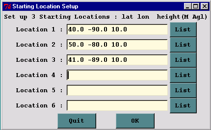
Although the setup of the concentration matrix calculation is similar to that of the trajectory matrix calculation, there is an additional option that can be set in the Advanced Menu configuration tab that changes the nature of the concentration output file to produce a source-receptor matrix. This will be discussed further below. The matrix calculation is a way to set up the CONTROL file for multiple starting locations that may exceed the GUI limit under the Concentration Setup menu tab. Hundreds or thousands of starting points may be specified. The Run Matrix menu tab first runs a program that reads the CONTROL file with three starting locations and then rewrites the same CONTROL file with multiple locations. The multiple locations are computed from the number of starting points that fall in the domain between starting point 1 and starting point 2, where each new location is offset is the same as that between starting locations 1 and 3. For instance, if the original control file has three starting locations: #1 at 40N, 90W; #2 at 50N, 80W, and #3 at 41N, 89W; then the matrix processing results in a Control file with 121 starting locations, all one degree apart, all between 40N 90W and 50N 80W.

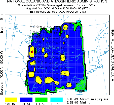
In the normal model execution mode, the concentration contributions from multiple sources are summed on the concentration grid, hence it is not possible to determine the fraction of the material comes from each source location. This can be seen in the illustration below using the above configuration for the first 12 hours of the sample case.
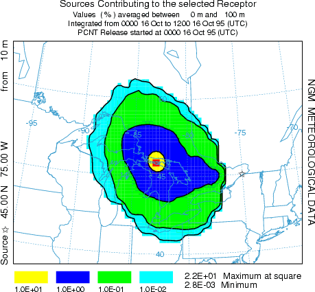
However, if the "Matrix" conversion module is checked in the Advanced Concentration Configuration menu tab, then the multiple source simulation maintains the identity of each source in the concentration output file. The Display Matrix menu tab permits extraction of information for individual sources or receptors from this special concentration output file. The results of the same simulation are shown in the illustration below. In this case the receptor check-box was set and the receptor location was identified as 45.0,-75.0 with normalization. Therefore the graphic illustrates the fractional contribution of each region to the first 12 hour average concentration at the designated receptor.
The following table illustrates the HYSPLIT matrix configuration. Emissions occur from each of N source locations and the receptors represent the concentration grid of M nodes. A single concentration output file is produced where each source contributes to its own concentration grid of M receptors. When selecting a "source" display, the M columns from the source location (row) represent the downwind concentration pattern for that source. When the receptor location (column) is selected, the contours represent the concentrations (each row of that column) contributing to that receptor from each of the source locations. Source and receptor grids should be of comparable resolution.

There are two other more quantitative approaches to source-attribution available through the menu and both require the measured sampling data. In the first approach, menu system is used to configure the model to execute a script to run multiple iterations of the upwind dispersion calculation for periods that correspond with individual measured sampling data. The results are then overlaid to determine the most likely source region. In the second approach, the menu system is used to solve the source-receptor coefficient matrix for the source term vector given a measured data vector and where the matrix values are the dilution factors for each source-receptor pair as described above.
Geolocation
In a manner similar to the daily menu, the dispersion model can be run for multiple simulations in time but where each simulation is configured as an adjoint calculation (backward in time) from measured concentration data points. More information on this procedure can be found in the geolocation help menu.
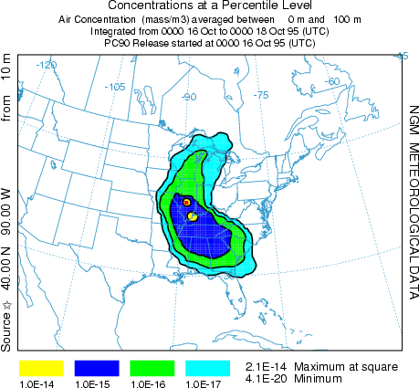
The ensemble form of the model, an independent executable, is similar to the trajectory version of the ensemble. The meteorological grid is offset in either X, Y, and Z for each member of the ensemble. The model automatically starts each member on a single processor in a multi-processor environment or cycles through the simulations on one processor. The calculation offset for each member of the ensemble is determined by the grid factor as defined in the Advanced Concentration Configuration Tab. The default offset is one meteorological grid point in the horizontal and 0.01 sigma units in the vertical. The result is 27 ensemble members for all offsets. The normal Setup Menu tab is used to configure the CONTROL file. Note that if fewer than 27 processors are available, the ensemble configuration menu permits starting the calculation at any ensemble member number within the valid range. Because the ensemble calculation offsets the starting point, it is suggested that for ground-level sources, the starting point height should be at least 0.01 sigma (about 250 m) above ground. The model simulation will result in 27 concentration output files named according the file name setting in the control file "{cdump}.{001 to 027}" with a suffix equivalent to the ensemble member number. On a single processor system, the calculation may take some time to cycle through all the members. The menu will be locked until the simulation has completed. A message file window will open after termination. Computational progress may be monitored by noting the generation of new concentration output and message files with the ensemble number suffix in the /working directory. The concentration output from each member can be displayed through the concentration display menu tab. However, to display the probabilities associated with the multiple simulations, it is necessary to pre-process the data through the Display Ensemble menu tab. Using the default configurations for the sample simulation, the illustration below represents the 90th percentile concentrations aggregating all four output time periods. For instance the blue contour in this 90th percentile plot represents the region in which only 10% of the ensemble members have air concentrations greater than 10-15. If the meteorological ensemble is run through a script or batch file instead of the GUI, the executable, with a command line parameter of the member number, must be run once for each of the 27 members.
Another ensemble variation is the turbulence option, which also creates 27 ensemble members, but due to variations in turbulence rather than variations due to gradients in the gridded meteorological input data. The variance ensemble should only be run in the 3D particle mode and with fewer particles, in proportion to the number of ensemble members to the number of particles required for a single simulation. For instance, if 27,000 particles are required to obtain a smooth plume representation, then each member should be run for 1000 particles. Normally the same random number seed is used when computing the turbulent component of the particle motion. However, in the variance ensemble, the seed is different for each member, resulting in each member representing one realization of the ensemble.
The variance ensemble can also be used to determine the number of particles required for a simulation, by progressively increasing the particle number until the variance decrease with increasing particle number is no longer significant. Because the number of particles required for a simulation increases with increasing distance from the source, a typical downwind receptor location needs to be selected and then by using the box plot display option, the concentration variability (max-min range) can be estimated and then determining when the decrease in range is no longer cost effective (in terms of computational time) with increasing particle number.
The physics ensemble is created by running a script that varies in turn the value of one namelist parameters from its default value. These are the parameters defined in the file SETUP.CFG and normally set in the Advanced Concentration Configuration menu tab. If the namelist parameters have not been defined through the menu, then the default values are assigned. In this first iteration, the GUI menu permits no deviation from the values assigned by the script. The entry box is for information purposes only to show the progress of the computation.
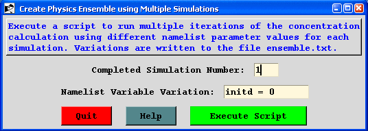
A summary of the current 15 ensemble variations is also written to the file ensemble.txt showing the name of the concentration output file and member variation. Check the advanced menu help files for more information on each variable.
Ensemble reduction based on minimization of square error
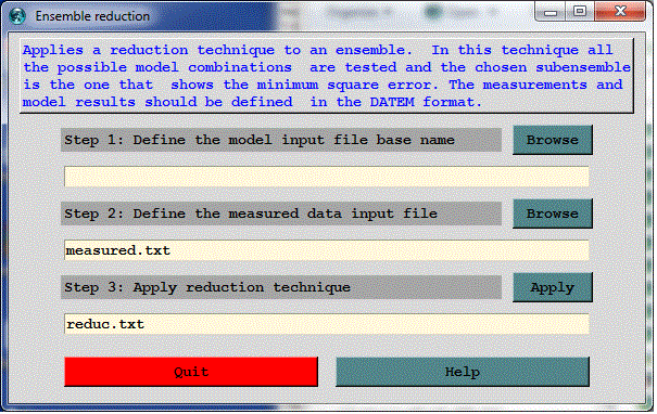
Over the last few years, the use of dispersion model ensembles has been an increasingly attractive approach to study atmospheric transport in the lower troposphere. Ensembles are constructed either by combining multiple numerical weather prediction simulations, different dispersion models, introducing variations in a particular model�s physics parameterizations or different combinations of these variations. The determination of the optimum number of multi-model members and/or individual model physical features to vary is the primary difficulty to overcome when constructing these dispersion simulation ensembles. In many studies the ensemble members just consisted of the available model outputs from different research groups regardless of the model characteristics or the result of performing an arbitrary number of runs with different configurations by individual researchers. Both approaches increase the possibility of redundancy which means that many of the ensemble members may not be much different from each other. In general, any ensemble might contain redundant information that overemphasizes certain transport and dispersion features that can be inaccurate. For example, perhaps a sub-group of members all use the same meteorological data, which might not be as accurate as another meteorological data set that is used by fewer members. Therefore, simply due to a dependency among many of the members to the same data, the ensemble including these members would be less accurate than one constructed from an ensemble based upon only the independent members. Conversely, independence among ensemble members does not necessarily imply that the reduced group of runs will be more accurate than the full ensemble because, by chance, the later could be also over emphasizing redundant members that happen to be more accurate. Consequently, we can apply reduction techniques with the intent to produce more accurate results than those obtained with the full ensemble and therefore requiring fewer computing resources. Solazzo and Galmarini (2014) demonstrated that an ensemble can be reduced by optimizing the skills of the mean taken among all the possible subsets of ensemble members. Following this methodology we calculate the average of all the possible model combinations composed by an increasing number of sub ensemble members up to the total number of members of the full ensemble and estimate their MSE. Furthermore, if M is the total number of ensemble members and n is the number of sub ensemble members, then the number of possible combinations is given by M!/(n!*(M-n)!). In other words, if our ensemble has, say, 24 members we will combine them in 276 pairs, 2024 trios, 10626 quartets, etc. and determine which combination provides the minimum MSE. The reduction technique is applied by running a postprocessing program that reads the different ensemble member outputs along with the measured data (all in DATEM format) and calculates the minimum square errors for each possible model output combination.
E. Solazzo, S. Galmarini, 2014. The Fukushima-137Cs deposition case study: properties of the multi-model ensemble, Journal of Environmental Radioactivity, Available online 22 March 2014, ISSN 0265-931X, http://dx.doi.org/10.1016/j.jenvrad.2014.02.017
Global
The global simulation is a HYSPLIT "grid-in-plume" option, in which the Lagrangian particle mass can be transferred to a global Eulerian model after a designated number of hours. Lagrangian and Eulerian dispersion and transport can occur simultaneously. Each model has its own output grid. The advantage of this approach is that at times very long-range calculations may require too many particles to properly represent the pollutant distribution. In this way it is possible to take advantage of the the more precise Lagrangian approach near the source and the more computationally efficient Eulerian computation at the hemispheric and global scales. More information on how to configure this simulation can be found in the global model help menu.
A model for the emission of PM10 dust has been constructed (Draxler, R.R, Gillette, D.A., Kirkpatrick, J.S., Heller, J., 2001, Estimating PM10 Air Concentrations from Dust Storms in Iraq, Kuwait, and Saudi Arabia, Atmospheric Environment, Vol. 35, 4315-4330) using the concept of a threshold friction velocity which is dependent on surface roughness. Surface roughness was correlated with geomorphology or soil properties and a dust emission rate is computed where the local wind velocity exceeds the threshold velocity for the soil characteristics of that emission cell. A pre-processing program was developed that accesses the HYSPLIT land-use file over any selected domain and modify the input CONTROL file such that each emission point entry corresponds with a "desert" (active sand sheet) land-use grid cell. The original PM10 flux equation was replaced by a more generic relationship (Westphal, D.L., Toon, O.B., Carlson, T.N., 1987. A two-dimensional numerical investigation of the dynamics and microphysics of Saharan dust storms. J. Geophys. Res., 92, 3027-3029).
The dust storm simulation is configured in the same way as the matrix calculation in that it is necessary to define three source locations, the first two representing the limits of the domain, and the third defining the emission grid resolution. The pre-processor then finds all emission points within that domain that have a desert category and modify the CONTROL file accordingly. The dust box must be checked in the advanced configuration menu to compute the PM10 emission rate. As an example, we can configure the model to run the large Mongolian dust storm of April 2001. An animation of the calculation results can be downloaded. To run the same simulation it will be necessary to obtain the first two weeks of northern-hemisphere meteorological analysis data (FNL.NH.APR01.001). A pre-configured CONTROL file (dust_conc) should be retrieved from the working directory. The CONTROL file defines the emission domain by the three starting locations: 35N-90W to 50N-120W with the grid increment to 36N-91W. There is no point in defining an emission grid of less than one-degree resolution because the resolution of the land-use data file is one-degree and the meteorological data is closer to two-degrees. Once the model is setup for the simulation, including the dust check-box in the configuration menu, execute the model from the Special Simulations / Run Dust Storm menu tab. Not available through the GUI, but another option in the SETUP.CFG namelist file, is the emission threshold sensitivity factor, which normally defaults to one. For instance, adding the line P10F=0.5 to the namelist file, would cause dust emissions to occur at half the normal threshold velocities. Starting the model will cause the window shown below will open to indicate the revision of the CONTROL file.
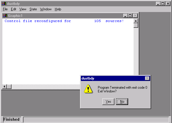
The message indicates that the initial 3-location CONTROL file was reconfigured by the dustbdy program for 105 source locations. That means in the domain specified, 105 one-degree latitude-longitude grid cells were found to have a desert land-use category. If none are found, then the CONTROL file is deleted to prevent model execution. Click on Yes or No to continue - yes just deletes the window. The model execution will then start. PM10 pollutant dust particles are only emitted from those 105 cells where the wind speed exceeds the emission threshold. Therefore it is possible to have simulations with no emissions. An example of the output after 24 hours simulation time is shown in the illustration below.
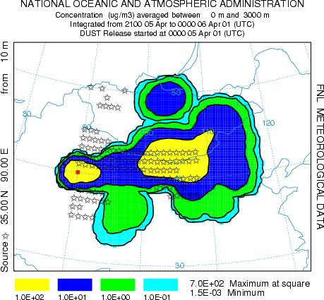
The concentrations represent a 3-hour average from 21 to 24 hours after the start of the simulations. It is not possible to say exactly from when or where particles are emitted except to note that the 105 potential source locations are shown. The emission algorithm emits in units of grams, but the in configuring the concentration display, the units were changed to ug by defining a conversion factor of 106. Maximum concentrations are on the-order-of 100, but the layer was defined with a depth of 3 km to facilitate comparison with satellite observations. The simulation could be rerun with a smaller layer to obtain concentrations more representative of near-ground-level exposures.
Daughter Products
A nuclide daughter product module has been incorporated into HYSPLIT. Given a chain of decay from a parent nuclide, the model can calculate the additional radiological activity due to in-growth of daughter products using the Bateman equations. Information about the available daughter products available in the model can be found in ../auxiliary/ICRP-07.NDX. More information on how to configure this simulation can be found in the daughter product help menu.