Concentration / Display / Ensemble / View Map

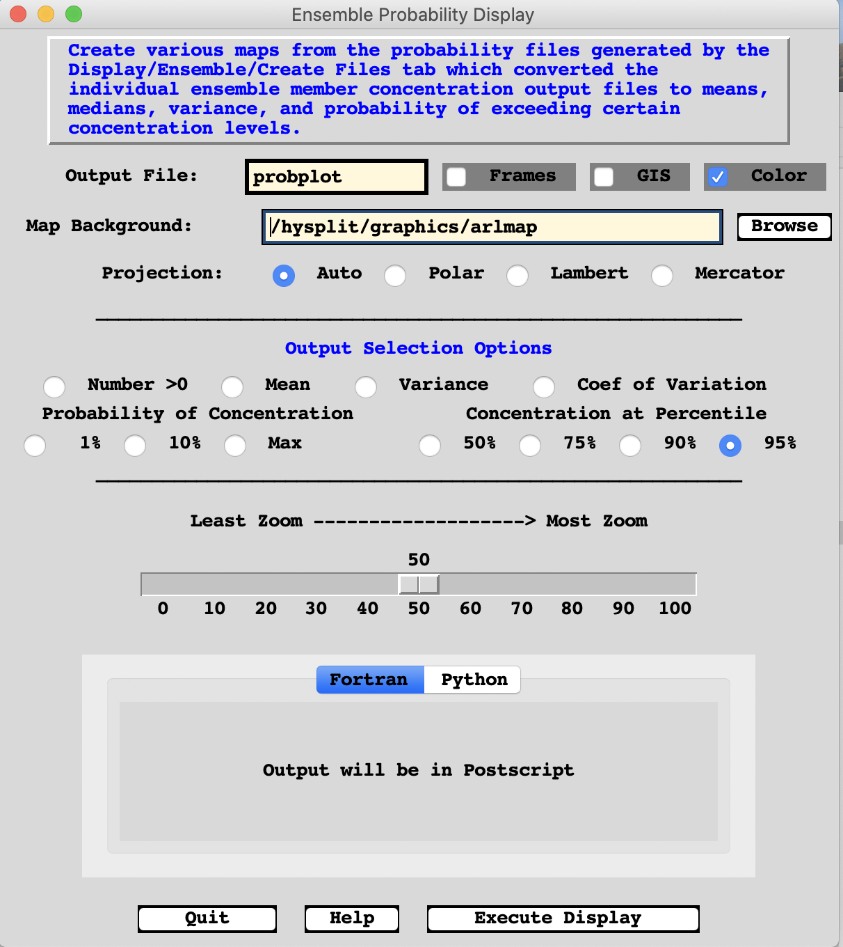
Multiple concentration output files from the ensemble or variance dispersion simulation should have been previously processed in the ensemble Create Files tab of the display menu. This step would have created fourteen probability output files in the working directory. These files are used to generate all graphics. The selected files are then plotted using concplot according to the menu options. An illustration of the View map menu is shown below.

The menu includes some of the standard display program (concplot) mapping choices, such as background file, output file name, zoom factor, and employment of FORTRAN- or Python-based implementation.

The menu permits a choice of six different ensemble output display options:

1. The number of ensemble members at each grid point with concentrations greater than zero shows the spatial distribution of the number of members (cnumb).
2. The mean concentration of all ensemble members (cmean).
3. The variance or the mean square difference between individual members and the mean (cvarn).
4. The coefficient of variation of all ensemble members expressed as the √Cvarn*100/Cmean (ccoev).
5. The probability of concentration produces contours that give the probability of exceeding a fixed concentration value at one of three levels: 1% of the maximum concentration (cmax01), 10% of the maximum (cmax10), and the maximum concentration (cmax00). The concentration level for the probability display is shown on the graphic with the pollutant identification field set to something like C14, where 14 represents the concentration to the power of 10^-14.
6. The concentration at percentile levels shows the concentration contours of areas where concentrations will be exceeded only at the given probability level. Although several output levels are computed, the probability level choices through the menu are limited to 50, 90, and 95th percentiles (prob[75|90|95]).