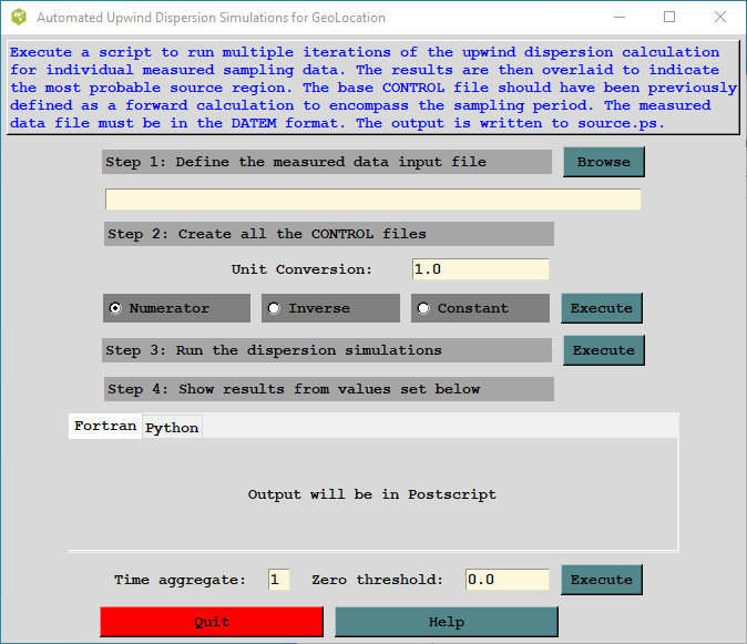
Summary: This menu is used to configure the model to execute a script to run multiple iterations of the upwind dispersion calculation for periods that correspond with individual measured sampling data. The model results are then overlaid to indicate the most probable source regions. The CONTROL file should have been previously defined for a forward calculation that corresponds to the sampling period of the measured data. The measured data file must be in the DATEM format. The output is written to the source.html HTML file in the working directory.
Step 1: defines the measured data input used in this series of calculations. The dispersion model is run in its backward mode, from each of the sampling locations, with a particle mass proportional to the measured concentration and with the particles released over a period corresponding to the sample collection period. Sampling data files are in the ASCII text DATEM format. The first record provides some general information, the second record identifies all the variables that then follow on all subsequent records. There is one data record for each sample collected. All times are given in UTC. The DATEM sampling data records have the following format:
An sampling data file which is used in the following calculations can be found in examples\matrix\measured.txt. These synthetic measurements (units = picograms per cubic meter) were created from a model simulation using the sample meteorological data in the working directory for a hypothetical 6-minute (0.1 hr) duration release of 10 kg of material from 40N 80W starting at 1200 UTC 16 Oct 1995.
Step 2: creates one CONTROL.{xxx} file for each sample (data record) in the previously defined measured data file. The CONTROL files are numbered sequentially from 001 to a maximum of 999, the current limitation of the program used to overlay the simulation results. The individual simulation control files are created from the current configuration shown in the concentration setup menu. The examples\matrix\control_geo file and the examples\matrix\setup_geo file templates should be retrieved into the setup and configuration menus. The template is a configuration for a forward simulation that encompasses the entire sampling period, with output intervals that correspond with the sampling intervals of the measured data. Essentially a configuration that could be used to predict the concentrations at the measurement locations if you knew the actual location and amount of the release. This step calls the pre-processor program (dat2cntl) which uses the configuration as a template to design each individual simulation CONTROL file. Each of these CONTROL files is configured as a backward simulation for the entire computational period, with the particle release occurring over the time of the sample collection. This insures that each simulation output file will contain an identical number of output periods, regardless of the time of the particle release. The template control file should have all key parameters specified such as the starting time and the center of the concentration grid. Do not use the zero default options in the CONTROL file, explicitly set all variables. All simulations must be identical.
There are three solution options. The default option Numerator, discussed above, uses the measured concentration in the numerator as the emission rate, resulting in a source sensitivity map weighted by the measured data. Checking the Inverse box sets the source term as the inverse of the measured concentration. This modeling scenario is comparable to the S = R/D situation described in the matrix solution help file>. In this case the model is computing D/R, where D is the dilution factor computed by the model and R is the measured concentration. The source term for the calculation is set to 1/R and only measurements where R is greater than or equal to zero are considered. Therefore, the resulting output (D/R) is an estimate of the inverse of the source term (1/Q) required to match the measured value for that simulation. A unit conversion factor needs to be set to output the appropriate mass units. The last option is to set the Constant radiobutton which results in the emission rate equal to the value set in the constant conversion factor entry box. In this type of simulation, each sample gets equal weight and the model results may be used to determine the optimal emission rate required to match the measured data.
Step 3: sequentially runs the dispersion simulations starting with CONTROL.001 through the last available control file. Each simulation uses the same namelist configuration shown in the menu. Note that a simulation is run for each measurement, high values as well as zero measurements. Non-zero measurements result in an hourly emission rate equal to the measurement value, while zero measurements are set to a very small, but non-zero value. In the context of this particular calculation, the intent of the source-attribution is primarily to determine the source location and perhaps its timing rather than estimating the emission rate from the measurements. Determination of emission rates should be done through the matrix menu option. The measurement data are only used to weight the source-sensitivity results for each simulation. Depending upon the model setup and configuration, simulation wall-clock times may vary considerably. Each simulation output results in a binary concentration file and message file with the same run number suffix as the control file.
Step 4: shows the multiple simulation results by averaging the source sensitivity function at each grid point over all the simulations. The dispersion model result of the upwind (backward) calculation looks similar to the air concentration field of the downwind (forward) calculation, but represents not concentration, but the source regions that may contribute to the air concentration at the measurement location from which the upwind calculation was started. There are two optional parameters that influence the output graphic. The time aggregate default is one, meaning that each sampling period is represented by one graphic. In the example calculation shown below, the source sensitivity function is shown for the last time period of the simulation and represents the average of all the simulations (zero and non-zero) from different time periods valid for that 6-hour sampling period. A time aggregation value of 5 would average the results from all 5 time periods into one graphic. The zero threshold value can be used eliminate the very low level contours that result from the zero-emission simulations. For instance, selecting a value of 1.0E-15 (1/1000 of a pg/m3) would set to zero any grid points less than that value.
The comparable graphic for the inverse calculation is shown below for the mean emission values for 15 simulations that had non-zero measurements. Before creating control files for the inverse simulation, previous control files should be deleted to avoid mixing together the two types of simulations. For this example, the measured data file has 15 non-zero measurements and 30 zero measurements and the units conversion factor should be set to 1.0E-15 to go from pg to kg. The resulting interpretation of the graphic is that the central contour (value = 1) indicates an average emission of 1 kg in that region. The outermost contour (0.01) would require 100 kg to be released to match the measured data. Greater dilution (D is smaller) require greater corresponding emissions to match the measured data.