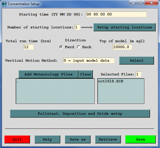
The initial setup menu for the concentration model is identical to the trajectory setup run menu in terms of starting time, location, and meteorology. These items will not be discussed again except to note the differences when applied to a dispersion simulation. The meaning of the entries in the CONTROL file that correspond to this setup menu are discussed in more detail below and should be reviewed to appreciate how the change in the simulation type (from trajectory to concentration) changes the meaning and context of the same input parameters. These parameters consist of the initial entries of the CONTROL file. The initial concentration setup menu is shown in the illustration below.
The entries in the Control file for air concentration simulations consist of four groups of input data. The first data group is almost identical to the trajectory simulation and is described in the next section. The other three groups define the pollutant emission characteristics, the concentration grid in terms of spacing and integration interval, and the pollutant characteristics relevant to computing deposition and removal processes. These latter three entries are accessed through the "Pollutant, Deposition, and Grids Setup" tab. Each of the these sections contains a more detailed description of the input parameters as well as the corresponding CONTROL file values that need to be set for command line simulations.
The concentration model input control file can be created using any text editor. However if the GUI is not being used, it would be easier to let the model create the initial file based upon standard output prompts. These are described in more detail below. When data entry is through the keyboard (a file named CONTROL is not found), a STARTUP file is created. This contains a copy of the input, and which later may be renamed to Control to permit direct editing and model execution without data entry. If you are unsure as to a value required in an input field, just enter the forward slash (/) character, and the indicated default value will be used. This default procedure is valid for all input fields except directory and file names. An automatic default selection procedure is also available for certain input fields of the CONTROL file when they are set to zero. Those options are discussed in more detail below. Each input line is numbered (only in this text) according to the order it appears in the file. A number in parenthesis after the line number indicates that there is an input loop and multiple entry lines may be required depending upon the value of the previous entry.
1- Enter starting time (year, month, day, hour, (minute, optional))
Default: 0 0 0 0
Enter the two digit values for the UTC time that the calculation is to start. Use 0's to start at the beginning (or end) of the file according to the direction of the calculation. All zero values in this field will force the calculation to use the time of the first (or last) record of the meteorological data file. In the special case where year and month are zero, day and hour are treated as relative to the start or end of the file. For example, the first record of the meteorological data file usually starts at 0000 UTC. An entry of "00 00 01 12" would start the calculation 36 hours from the start of the data file.
The minute field is optional. If the minute field is not present, then the default value of 0 will be used.2- Number of starting locations
Default: 1
Single or multiple pollutant sources may be simultaneously tracked. The emission rate that is specified in the pollutant menu is assigned to each source. If multiple sources are defined at the same location, the emissions are distributed vertically in a layer between the current emission height and the previous source emission height. The effective source will be a vertical line source between the two heights. When multiple sources are in different locations, the pollutant is emitted as a point source from each location at the height specified. Point and vertical line sources can be mixed in the same simulation. The GUI menu can accommodate multiple simultaneous starting locations, the number depending upon the screen resolution. Specification of additional locations requires manual editing of the CONTROL file. Area source emissions can be specified from an input file: emission.txt. When this file is present in the root directory, the emission parameters in the CONTROL file are superseded by the emission rates specified in the file. More information on this file structure can be found in the advanced help section.
3(1)- Enter starting location (lat, lon, meters, Opt-4, Opt-5)
Default: 40.0 -90.0 50.0
Position in degrees and decimal (West and South are negative). Height is entered as meters above ground level unless the mean-sea-level flag has been set.
The optional 4th (emission rate - units per hour) and 5th (emission area - square meters) columns on this input line can be used to supersede the value of the emission rate (line 12-2) when multiple sources are defined, otherwise all sources have the same rate as specified on line 12-2. The 5th column defines the virtual size of the source: point sources default to "0".
4- Enter total run time (hours)
Default: 48
Sets the duration of the calculation in hours. Backward calculations are configured by setting the run time to a negative value. See the discussion in the advanced help section on backward "dispersion" calculations.
5- Vertical motion option (0:data 1:isob 2:isen 3:dens 4:sigma 5:diverg 6:msl2agl 7:average 8:damped)
Default: 0
Indicates the vertical motion calculation method. The default "data" selection will use the meteorological model's vertical velocity fields; other options include isobaric, isentropic, constant density, constant internal sigma coordinate, computed from the velocity divergence, a special transformation to correct the vertical velocities when mapped from quasi-horizontal surfaces (such as relative to MSL) to HYSPLIT's internal terrain following sigma coordinate, and a special option (7) to spatially average the vertical velocity. The averaging distance is automatically computed from the ratio of the temporal frequency of the data to the horizontal grid resolution.
6- Top of model domain (internal coordinates m-agl)
Default: 10000.0
Sets the vertical limit of the internal meteorological grid. If calculations are not required above a certain level, fewer meteorological data are processed thus speeding up the computation. Trajectories will terminate when they reach this level. A secondary use of this parameter is to set the model's internal scaling height - the height at which the internal sigma surfaces go flat relative to terrain. The default internal scaling height is set to 25 km but it is set to the top of the model domain if the entry exceeds 25 km. Further, when meteorological data are provided on terrain sigma surfaces it is assumed that the input data were scaled to a height of 20 km (RAMS) or 34.8 km (COAMPS). If a different height is required to decode the input data, it should be entered on this line as the negative of the height. HYSPLIT's internal scaling height remains at 25 km unless the absolute value of the domain top exceeds 25 km.
7- Number of input data grids
Default: 1
Number of simultaneous input meteorological files. The following two entries (directory and name) will be repeated this number of times. A simulation will terminate when the computation is off all of the grids in either space or time. Calculations will check the grid each time step and use the finest resolution input data available at that location at that time. When multiple meteorological grids have different resolution, there is an additional restriction that there should be some overlap between the grids in time, otherwise it is not possible to transfer a particle position from one grid to another. If multiple grids are defined and the model has trouble automatically transferring the calculation from one grid to another, the sub-grid size may need to be increased to its maximum value.
While not available in the GUI, if the user is creating the CONTROL file themselves, two numbers can be specified here: the first being the number of unique grids and the second being the number of files in each grid. For example, an entry of 2 12 would mean that there are met files for 2 different grids (e.g., a regional and a global grid), and that there are 12 files being specified for each grid. The grids should be specified in order of resolution, with the highest resolution grids (i.e, the smallest horizontal spacing between grid points) being specified before lower resolution grids. The two entries for each file (directory and filename) are repeated for each file in the first grid, and then for each file in the second grid, and so on, for any subsequent grids. Note that the same number of files are required for each grid in this approach. Without the use of this approach (i.e., when only one number is specified) the maximum number of files that can be used in the simulation is relatively small, but with this second approach, a much larger number of files can be used in the simulation.
8(1)- Meteorological data grid # 1 directory
Default: ( \main\sub\data\ )
Directory location of the meteorological file on the grid specified. Always terminate with the appropriate slash (\ or /).
9(2)- Meteorological data grid # 1 file name
Default: file_name
Name of the file containing meteorological data. Located in the previous directory.