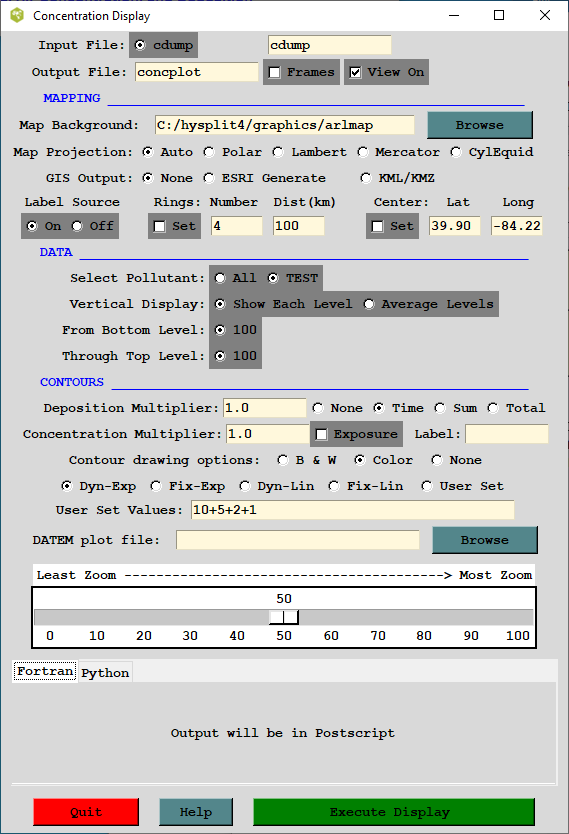
The concentration model generates a binary (big-endian) output file on a regular latitude-longitude grid, which is read by the other programs to produce various displays and other output. The plotting program, concplot, can be accessed through the GUI, which is shown in the illustration below, or it can be run directly from the command line. Most, but not all, of the command line options are available through the GUI.
Normally only one input file is shown, unless multiple files have been defined in the Concentration Setup Run menu. The default output file name is shown and unless the box is checked all frames (time periods and/or levels) will be output to that one file. The program uses the map background file, arlmap, which by default is located in the \graphics directory. Other customized map background files could be defined. Some of these higher resolution map background files are available from the HYSPLIT download web page. This plotting program also supports the use of ESRI formatted shapefiles.
The GIS output option will create an output file of the contour polygons (latitude-longitude vectors) in two different format: the ESRI generate format for import into ArcMap or ArcExplorer, or XML formatted files packaged by Info-Zip for import into Google Earth.
For multiple pollutant files, only one pollutant may be selected for display by individual levels, or averaged between selected levels. These levels must have been predefined in the Concentration Setup menu. Multipliers can be defined for deposition or air concentrations. Normally these values would default to 1.0, unless it is desired to change the output units (for instance, g/m3 to ug/m3 would require a multiplier of 106).
Contours and color fill can be specified as black and white or color. The none option eliminates the black line defining contours and only leaves the color fill. This option is incompatible with GIS output options, which require computation of the contour vector. Contours can be determined DYNamically by the program, changing with each map, or FIXed to be the same for all maps. A user can set the contour scaling (difference between contours) to be computed on an EXPonential scale or a LINear scale.
A Python implementation of the concplot program is added to this distribution package. By default, the GUI uses concplot built from FORTRAN code. To use the Python implementation, select the Python tab near the bottom of the user interface before generating a plot.
The Postscript/SVG conversion program (concplot), found in the /exec directory with all other executables, reads the binary concentration output file, calculates the most optimum map for display, and creates the output file concplot.ps or concplot.html. Multiple pollutant species or levels can be accommodated. Most routine variations can be invoked from the GUI. More complicated conversions should be run from the command line using the following optional parameters:
concplot -[options (default)]
Selecting the ESRI Generate Format output creates an ASCII text file for each output time period that consists of the value and latitude-longitude points along each contour. This file can be converted to an ESRI Shapefile or converted for other GIS applications through the utility menu "GIS to Shapefile" ". The view checkbox would be disabled to do just the GIS conversion without opening the Postscript viewer. Selecting Google Earth will create a compressed file (*.kmz) for use in Google Earth; a free software package to display geo-referenced information in 3-dimensions. You must have the free Info-Zip file compression software installed to compress the Google Earth file and associated graphics. The Python implementation can take several formats. See the description for the --more-gis-options option below.
Selecting clampedToGround (0) positions the contoured concentrations flat on the Google Earth terrain, whereas selecting relativeToGround will generate 3D contours be extending the edges of the contours to the ground from the valid height of the concentration data.
= 0 - Represents the height (meters) below which no data will be processed for display. The level information is interpreted according to the display (-d) definition.
= 1 - All output levels that fall between the bottom and top display heights are shown as individual frames. A single level will be displayed if both bottom and top heights equal the calculation level or they bracket that level. Deposition plots are produced if level zero data are available in the concentration file and the display height is set to 0.
= 2 - The concentrations at all levels between the specified range are averaged to produce one output frame per time period. If deposition data is available and a plot is required in addition to the air concentrations, then the bottom height should be set to 0. Deposition is not averaged with air concentrations.
= 1 - A custom output format in which all the air concentrations have been converted to time-integrated units and vertically averaged for all levels between the bottom and top heights.
= 0 - All output frames (one per time period) in one file.
= 1 - Each time period is written to a file: concplot{frame number}.ps
= ( ) - Auto selection procedure draws four circles with the distance between them determined by the program algorithm.
= # - Specifies the number of circles with the default (50 km) distance interval.
= number:distance - specifies the number of circles and the distance interval between circles. For the special case of zero circles with a distance specified (e.g. -0:1500) the program will fix the map with the top and bottom edge at that distance from the center.
= 0 - Output in Postscript.
= 1 - Output in HTML containing Scalable Vector Graphics.
Note that this option is unavailable in the Python version.
= lat:lon - Forces the center of the map to be at the specific latitude-longitude point rather than the default source location. This is normally used in conjunction with the -g option to get the same map each time or when there are multiple source locations.
= Name of the binary concentration file for which the graphics will be produced. Default name {cdump} or user defined}.
The program first searches the local directory, then the ..\graphics directory for the name of the default map background file (arlmap). Set this parameter to select the directory/name of any map background file of compatible format or specify a special file of shape file file names.
The default plot symbol over the source location is an open star. This may be changed to any value defined in the psplot ZapfDingbats library. For instance a blank, or no source symbol would be defined as -l32
= 0 - No latitude or longitude lines are drawn on the map
= 1 - Latitude and longitude lines spacing is determined automatically
= 2:tenths - line spacing is determined by the given value in tenths
Normally the map projection is automatically determined based upon the size and latitude of the concentration pattern. Sometimes this procedure fails to produce an acceptable map and in these situations it may be necessary to force a map projection.
The default (1) prints the maximum and minimum values below the contours and plots a red square, the size of the concentration grid, at the location of the maximum concentration value. These can be turned off individually using this command line option. Note the +m rather than -m prefix.
= 0 - All time periods in the input file are processed.
= # - Sets the number of time periods to be processed starting with the first.
= #1:#2 - Processes time periods, including and between #1 and #2.
= [-#] - Sets the increment between time periods to be processed. For instance,
-n-6 would only process every 6th time period.
The name of the Postscript output file defaults to concplot.ps unless it is set to a {user defined} value. The Python implementation supports several formats beside postscript. See the description for the --more-formats option below.
The suffix defines the character string that replaces the default "ps" in the output file name. A different suffix does not change the nature of the file. It remains Postscript. The suffix is used in multi-user environments to maintain multiple independent output streams.
By defining the name of a text file in this field where the data values are defined in the DATEM format, the values given in the file will be plotted on each graphic if the starting time of the sample value falls within the averaging period of the graphic.
= 0 - No deposition plots are produced even if the model produced
deposition output.
= 1 - One deposition plot is produced for each time period.
= 2 - The deposition is summed such that each new time period represents
the total accumulation.
= 3 - Similar to =2, deposition is accumulated to the end of the simulation
and but only one plot is produced at the end.
= {Species Number} - Only one pollutant species may be displayed per plot sequence if multiple species were created during a simulation. However, an entry of "0" will cause all species concentrations to be summed for display.
= 99999 - Represents the height (m) above which no data will be processed for display. The level is interpreted according to the display definition.
Defines the character string for the units label. Can also be modified using the labels.cfg file.
If the contour values are user set (-c4), then it is also possible to define up to ten individual contours explicitly through this option. For instance -v4+3+2+1, would define the contours 4, 3, 2, and 1. Optionally, a label and/or color (RGB) can be defined for each contour (e.g. -v4:LBL4:000000255+3:LBL3:000255255+2:LBL2:051051255+1:LBL1:255051255). To specify a color but not a label, two colons must be present (e.g. -v4::000000255).
Defines if the gridded concentration data are to be smoothed prior to contouring. For instance, a value of 1 means that each grid point value is replaced by the average value of 9 grid points (center point plus 8 surrounding).
= 1.0 - No units conversion.
= X - where {X} is the multiplier applied to the air
concentration input data before graphics processing.
= 1.0 - No units conversion.
= X - where {X} is the multiplier applied to the deposition
input data before processing.
= 50 - Standard resolution.
= 100 - High resolution map (less white space around the
concentration pattern)
Additional supplemental text may be added at the bottom of the graphic by creating a file called MAPTEXT.CFG, which should be located in the working directory. This is a generic file used by all plotting programs but each program will used different lines in its display. The file can be created and edited through the Advanced / Panel Labels menu tab. Units and title information can be edited by creating a LABELS.CFG file which can also be edited manually or through the Advanced / Border Labels menu tab.
Additional Concplot Command Line Options for Python Implementation
The following options are available only to the Python concplot.
--debug
Print debug messages. This is useful for developers to diagnose an issue.
--interactive
Enter interactive mode. Users can zoom in or move the plot area.
--more-formats=f1[,f2,...]
Specify one or more additional output format(s). This option supplements the output format specified by the -o option. For example, for -oa.ps --more-formats=pdf,png, three files would be produced, namely, a.ps, a.pdf, and a.png. Supported formats are eps, jpg, pdf, pgf, png, ps, raw, rgba, svg, svgz, and tif.
--more-gis-options=f1[,f2,...]
Specify one or more additional GIS output format(s). This option supplements the -a option. For example, with -a1 --more-gis-options=2, both ESRI Generate and Google Earth files will be created.
--source-time-zone
Display dates and times as a local time at the source location. If the option is not given, dates and times will be in Coordinated Universal Time (UTC).
--street-map[=n]
Show street map in the background. Currently, the option value n may take 0 (OPEN_STREET) or 1 (OPEN_TOPO). If no option value is used (i.e., --street-map), n = 0 will be used. This option overrides the -j option.
--time-zone=tz
Show dates and times as a local time at the given time zone tz. The time zone should be listed in the pytz Python package. For example, it could be US/Eastern, America/New_York, Etc/GMT-5, and so on.
ESRI Shapefile Map Background Files
Another mapping option would be to specify a special pointer file, (originally called shapefiles.txt, but now a suffix other than "txt" is permitted) to replace the map background file arlmap in the -j command line option (see above). Note -jshapefiles... rather than -j./shapefiles... is required. This file would contain the name of one or more shapefiles that can be used to create the map background. The line characteristics (spacing, thickness, color) can be specified for each shapefile following the format specified below: