2.1 Buoyant plume rise from fires (20 min) |
||||
 Previous |
|
|
 Next |
|


This example is a extension of the basic tutorial section on wild fire smoke. Review this case for background information. The plume rise was computed automatically during the HYSPLIT calculation because the heat release rate column in the EMITIMES file was non-zero and equal to 86 GW. The calculation will be re-run using 2X higher and lower multiples for the heat released.
- The SETUP.CFG namelist file to configured for a Gaussian plume simulation initially using 25,000 particles and with a 24 hour maximum duration to limit the maximum particle number:
initd = 3, Gaussian plume horizontal particle vertical khmax = 24, delete particles after 24h numpar = 25000, release 25000 particles maxpar = 50000, maximum particle number efile = 'EMITIMES', file with emission rate and fire heat - The emission section of the CONTROL file is set to a unit rate which will be replaced by the emission rate value in the EMITIMES file:
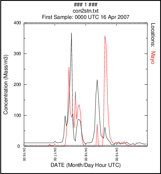
1 one pollutant PM25 defined as a PM 2.5 particle 1.0 default emission rate one unit per hour 72.0 emission duration in hours 00 00 00 18 00 emissions start at 1800 UTC on the 16th - The script simply loops through several different heat release rates, creating a new EMITIMES file for each simulation:
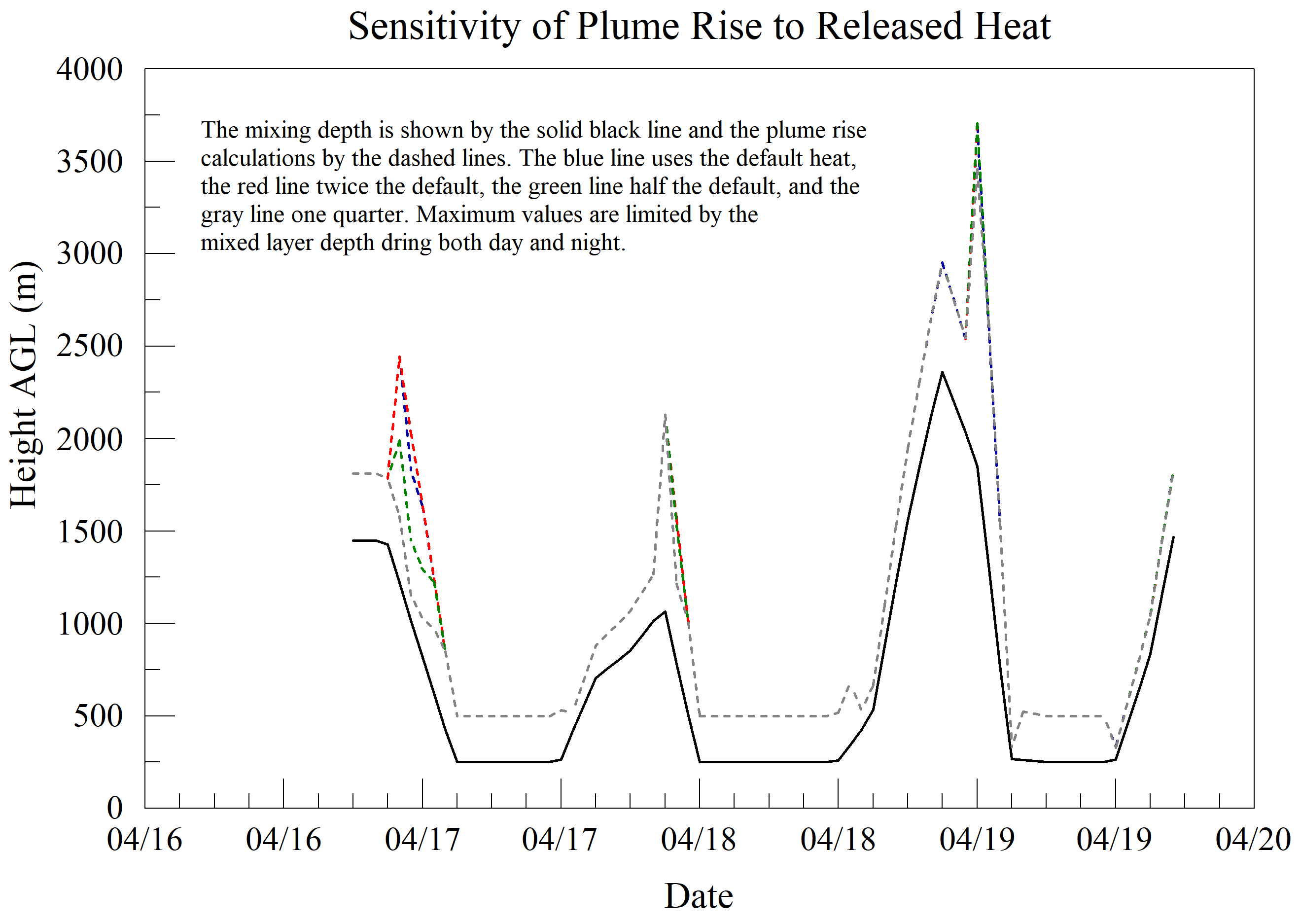
1: heat=0.215E+11 0.25 BASE 2: heat=0.430E+11 0.50 BASE 3: heat=0.860E+11 BASE case heat release rate 4: heat=1.720E+11 2.00 BASE - The base calculation (#3) should give the same plume picture as in the basic Tutorial:
concplot concentration plotting program -ismoke.bin HYSPLIT binary output file -uug set units label on map to micrograms -k1 draw contour lines between colors -c4 force contour levels -v500+200+100+50+20+10 set forced contours 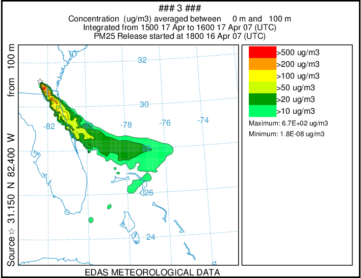
echo Mayo 30.2556 -81.4533 add Mayo site to samplers.txt file con2stn extract concentrations at station -ismoke.bin from binary input file -ocon2stn.txt values written to text file -r1 column format -ssamplers.txt list of stations to extract timeplot plot concentration time series -icon2stn.txt text input file of time varying values -s..\..\Tutorial\smoke\mayo_pm25.txt measurement data 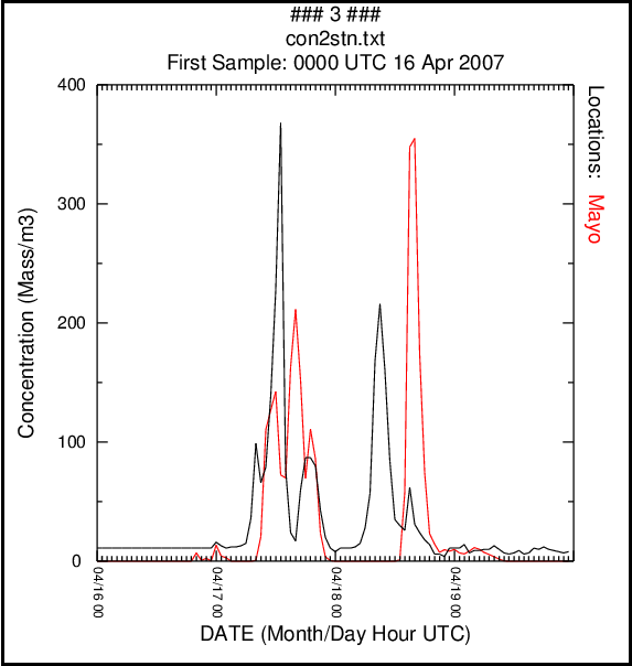
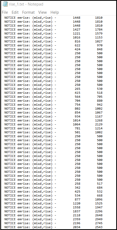
- After each HYSPLIT simulation has completed, each line of the MESSAGE file that contains the text mixd,rise is copied to a file. This line contains the average mixed layer depth (first data column) and plume rise (second data column) for all the computational particles the previous hour. For instance the first two days of the base calculation shows how the plume rise exceeds the mixing depth both at night and during the day. Stable mixing depths are limited to a minimum of 250 m unless a different minimum is defined in the namelist file. The HYSPLIT plume rise algorithm limits the plume rise to no higher than 25% of the mixed layer depth during neutral and unstable conditions and twice the mixed layer depth during stable conditions.
This is the primary reason why for larger fires the plume rise is insensitive to the heat. In this particular case, although the ground level concentration patterns were similar, the lower heat release rates showed a marginally better match with the concentration time series at Mayo.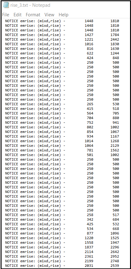
-
The plume rise sensitivity tests are summarized below showing that the 25% reduction case was the one to show the greatest influence with respect to ground-level air concentrations, but only during the first day.
Variations in released heat and resulting plume rise would make a excellent choice in constructing a dispersion ensemble for large fires. In the event detailed emission data are not available, it may also be possible to estimate air concentrations and hence the emission rate using a surrogate such as aerosol optical depth and assuming an extinction coefficient for smoke (~ 4 m2 g-1).