1.8 Simulate Smoky Nuclear Test |
||||
 Previous |
|
|
 Next |
|


In this example we model the transport and deposition of nuclear material from the Smoky nuclear test from Nevada in August 1957 and compare the results to measurements of dose rate over the Southwestern United States. A full description of the modeling effort can be found in the journal article Modeling the fallout from stabilized nuclear clouds using the HYSPLIT atmospheric dispersion model published in the Journal of Environmental Radioactivity in 2014. In the following sections below we review the key features of the script.
- Divide the initial nuclear cloud into 6 emission layers based on the top of the cloud with the activity distributed among particle sizes according to Glasstone and Dolan (1977) and proportioned as defined by Heffter (1969) in the figure:
and create the EMITIMES file for the simulation with 14 emission rates at each defined layer for the 14 particle sizes defined in the CONTROL file.
- Ensure that the emissions in the CONTROL file are set to zero to avoid using the wrong emission rate and set the emission time to 1 minute, which is when the nuclear cloud has been considered stabilized. In addition, define the initial 14 particle diameters, densities, and shapes, making sure the noble gas particle is defined with all zeroes:
14 14 pollutants (P001 - P013) including 1 for noble gases (NGAS) 0.0 emission rate units per hour 0.0166666666666667 emission duration in hours (1 minute) - Configure the SETUP.CFG namelist file to define five computational particle size bins centered about each defined particle size (NBPTYP=5) to provide a better distribution of particle sizes for calculating deposition. Also, the mass on a particle is removed once a particle is deposited assuming a probability of being deposited when in the deposition layer (ICHEM=5):
nbptyp = 5, number of redistributed particle size bins ichem = 5, probability of deposition numpar = 15000, particles released per emission cycle maxpar = 200000, maximum particle number efile = 'EMITIMES', file with emission rates - In the first post-processing step, the particle positions are displayed (every 3rd particle) every 2 hours of the 24 hour simulation:
parxplot horizontal and vertical particle plot -iPARDUMP particle position file -k1 color positions -n3 plot every third particle -jc:\hysplit4\graphics\arlmap map background file 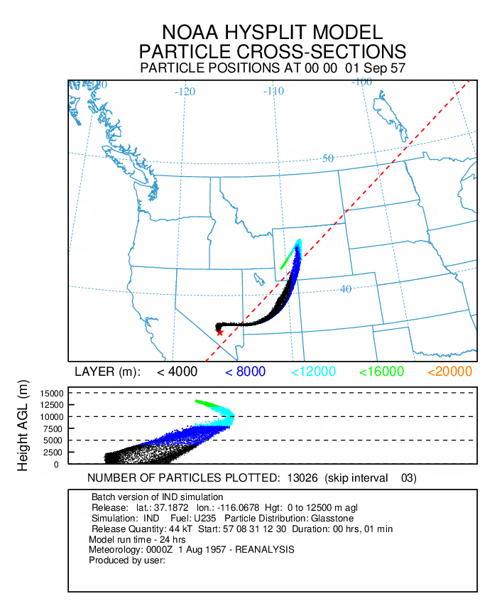
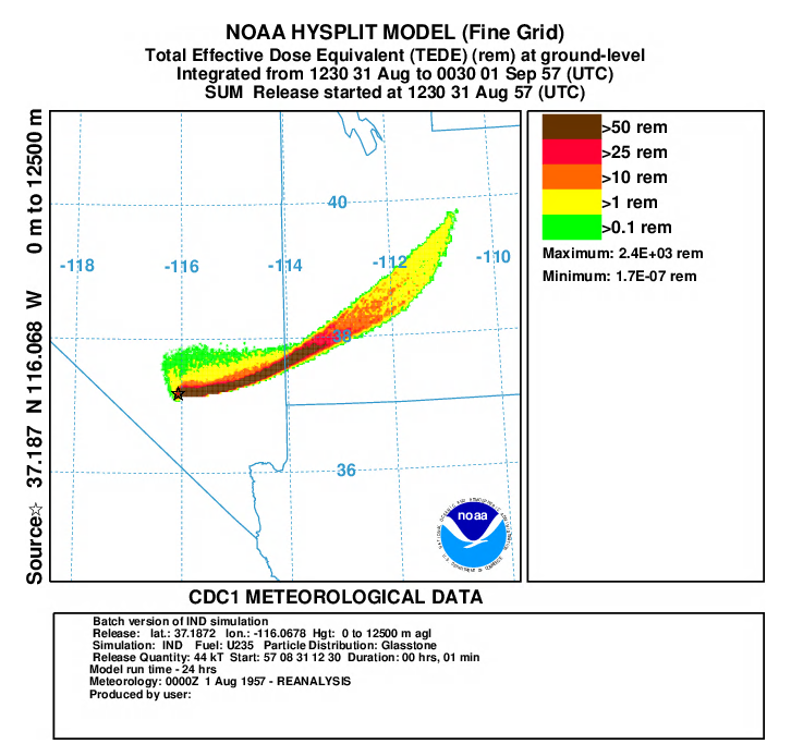
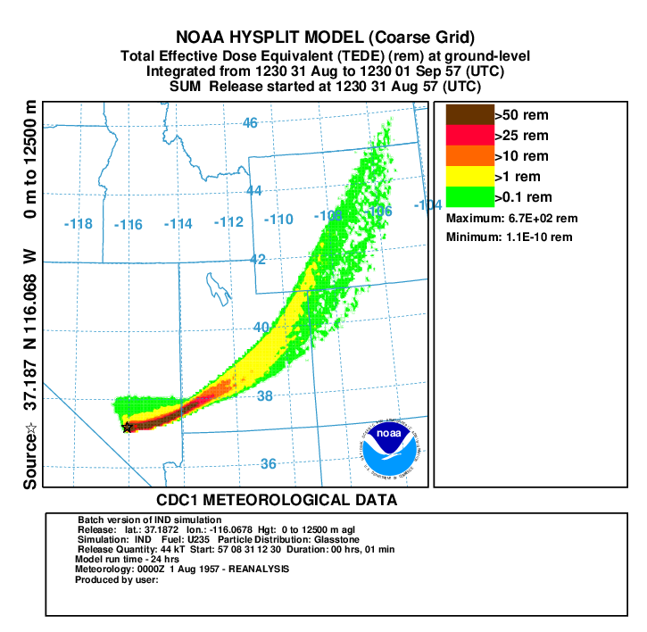
- In the second and third post-processing steps, we create a plots of the total effective dose equivalent (TEDE) on fine grid with a yield of 44 kT (repeat for coarse grid using binary file con1hc and dep1hc):
- First convert air concentration to dose:
con2rem convert air concentration to dose -icon1hf HYSPLIT binary input file for fine grid -oairdose.bin HYSPLIT binary output file for submersion and inhalation dose -a..\files\activity_IND.txt nuclear activity data for each specie -d1 output dose -e1 include inhalation dose in the calculation -y44 yield of weapon (kT) -f1 fuel type is U235 - Do the same for deposition:
con2rem convert air concentration to dose -idep1hf HYSPLIT binary input file for fine grid -odose96h.bin HYSPLIT binary output file for ground shine -a..\files\activity_IND.txt nuclear activity data for each specie -d1 output dose -y44 yield of weapon (kT) -f1 fuel type is U235 -x96 decay deposition for 96 hours (4-day dose) - sum the air doses over the grid prior to adding it to the dose from deposition:
concacc accumulate concentrations over all time periods -iairdose.bin HYSPLIT binary input file for submersion and inhalation dose -oaccaird.bin HYSPLIT binary output file for total air dose - add the submersion, inhalation and ground shine doses together:
concadd accumulate concentrations over all time periods -iaccaird.bin HYSPLIT binary output file for total air dose -bdose96h.bin HYSPLIT binary output file for 4-days of ground shine dose -otede.bin HYSPLIT binary output file for TEDE - display the results:
concplot concentration plotting program -itede.bin HYSPLIT binary output file -otede.ps Postscript output file -n1:12 plot first 12 maps (fine grid only) -s0 sum all species -c4 force contour levels -jc:\hysplit4\graphics\arlmap map background file -91 Force sample start time label to start of release -urem set units label on map -k2 do not draw contour lines between colors -v1::102000000+ set forced contours and colors 0.5::255000000+ 0.1::255102000+ 0.05::255204000+ 0.01::255255000 0.005::000000255
- First convert air concentration to dose:
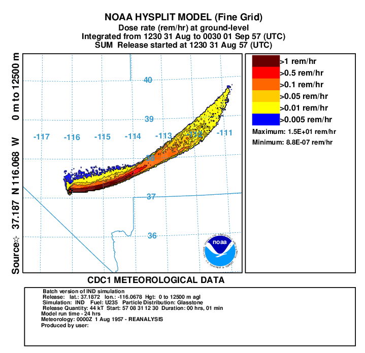
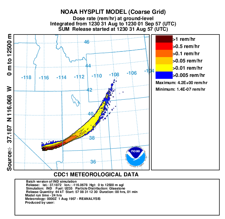
- In the next 2 steps, we create a plots of the dose rate (rem/h) from cloud shine and ground shine with all doses back decayed to 12 hours on fine grid to match measurements (repeat for coarse grid using binary file conc1hc):
- First convert air concentration to dose rate:
con2rem convert air concentration and deposition to dose rate -iconc6hf HYSPLIT binary input file for fine grid -odose6h.bin HYSPLIT binary output file for dose rate -a..\files\activity_IND.txt nuclear activity data for each specie -d0 output dose rate -e1 include inhalation dose in the calculation -y44 yield of weapon (kT) -f1 fuel type is U235 -z12 fixed integration time in hours - display the results:
concplot concentration plotting program -idose6h.bin HYSPLIT binary output file -odosert.ps Postscript output file -s0 sum all species -c4 force contour levels -jc:\hysplit4\graphics\arlmap map background file -91 Force sample start time label to start of release -urem/hr set units label on map -k2 do not draw contour lines between colors -v50::102051000+ set forced contours and colors 25::255000051+ 10::255102000+ 1::255255000+ 0.1::000255000
- First convert air concentration to dose rate:
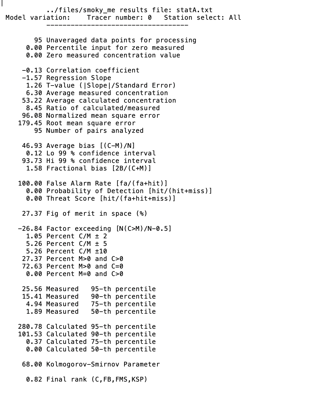
- In the last post-processing step we calculate statistics by comparing the modeled dose rates with measured dose rates on the coarse grid.
- First we sum the air dose over the grid before adding it to the dose from deposition:
concsum sum the air dose over the grid -idose1hc.bin HYSPLIT binary input file -odose1hcsum.bin HYSPLIT binary output file - next, convert the modeled doses to DATEM format and add to the measurements in DATEM format using c2datem:
c2datem convert model output to DATEM format -idose1hcsum.bin HYSPLIT binary output file -ohysplit_smoky.txt HYSPLIT DATEM output at for measurement locations -m..\files\smoky_meas.txt measured data file in DATEM format -c1000.0 conversion from Bq to mBq -xi interpolation - next, calculate statistics using statmain:
statmain calculate verification statistics -rhysplit_smoky.txt HYSPLIT DATEM output for measurement locations -d..\files\smoky_meas.txt measured data file in DATEM format -o1 write merged data file -t0 tracer character number -l10.0 contingency level (10%)
- First we sum the air dose over the grid before adding it to the dose from deposition:
In this example from the paper, using the higher resolution WRF meteorological data gave better results compared with measurements although both simulations had the plume too far to the north of the observed plume most likely due to the meteorology not capturing the initial wind direction to the southeast. Other researchers using other models also had the same problem with the modeled plume to the north of the observed plume. Try running this simulation with more particles to see if the you can improve the results.