2.5 Converting sulfur dioxide to sulfate (2 min) |
||||
 Previous |
|
|
 Next |
|


The HYSPLIT code has the capability to perform simple first-order linear conversions from one species to another. The conversion rates are specified in percent per hour. Multiple sequential conversion steps can be defined. This process is invoked using the ICHEM=2 namelist option and it only works when multiple species are defined on the same particle (MAXDIM>1). An example of this conversion process within HYSPLIT can be seen with the University of Hawaii's daily VOG forecasts for the Pu'u'O'o and Halema'uma'u vents of the Kilauea volcano in Hawaii. Recent observations show that the total SO2 emissions are nearly 5000 metric tons per day. Perhaps due to the tropical high temperatures and moisture content of the air, previous studies suggested that nearly 100% of the sulfur dioxide was converted to sulfate within the first hour. In this example, we will start with the same Eyjafjallajokull eruption used in the basic tutorial section.
- Starting with the original Eyjafjallajokull configuration, we will only perform a 12 h duration simulation, for a continuous release starting at 0000 UTC on April 16th. Note we have no information about actual SO2 emissions from Eyjafjallajokull so as a first guess we will use the rate from Kilauea, which converts to about 200,000 kg/h. Rather than four different particle sizes, we define only two species, one a gas, and the other a particle with a nominal settling velocity. For simplicity, we compute a simple tropospheric layer average air concentrations. The key elements of the CONTROL file are as follows:
../../Tutorial/volcano/ meteorology directory apr1420.bin data file SO2 sulfur dioxide 208333.3 emission rate kg per hour 12 emission duration in hours SO4 sufate 0.0 no emission 0.0 no emission - Only two lines are required in the SETUP.CFG namelist file, one turning on the linear conversion and the other defing that two pollutants will be assigned to each particle. Chemical conversions from one species to another can only occur on the same particle.
ichem = 2, turn on linear conversions maxdim = 2, dimension each particle with two mass species - The default conversion rate is 10% per hour with no mass conversion factor, which means one gram-mole of species one converts to one gram-mole of species two. However, if the file CHEMRATE.TXT is found in the working directory, then the conversion rates defined in that file will be used instead. In this example, the model will be run three times, for conversion rates of 5, 10, and 20% per hour. For instance, the contents of the file for the 20% per hour conversion:
- 1 2 0.20 1.5
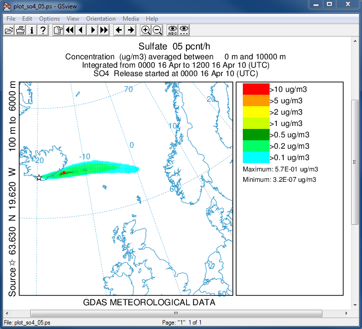
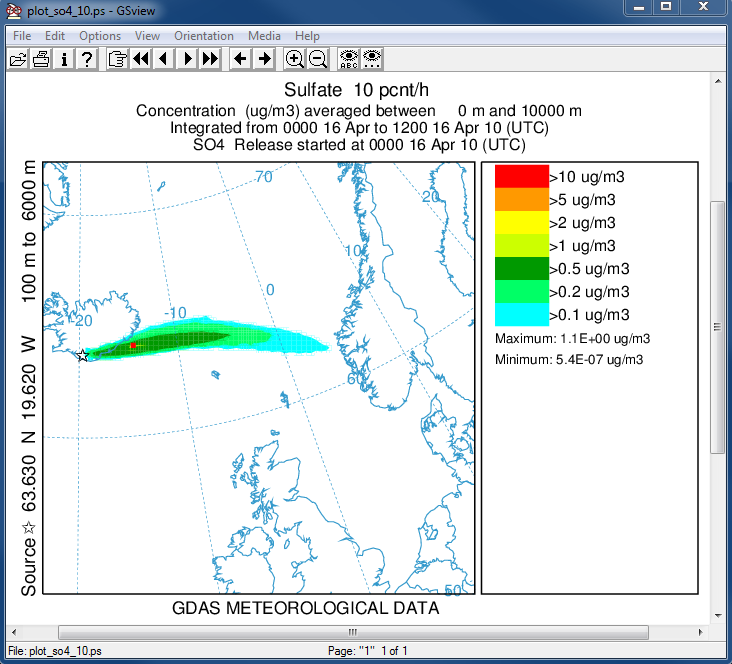
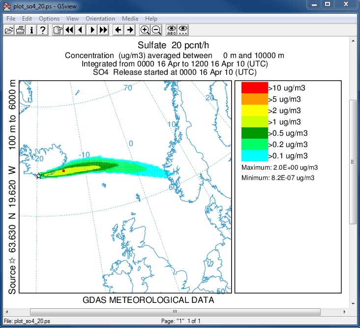
converts species #1 to #2 at 0.20 per hour, increasing the mass of species #2 by a factor of 1.5 with each conversion. The mass adjustment is required because converting from SO2 to SO4 picks up an additional O2. The molecular weight goes from 64 g/Mol to 96 g/Mol or a ratio of 1.5 with each conversion. - Once the simulation is completed the 12-h average plume graphic is displayed for each species. For sulfate, display units are typically mass over volume, which is already the native unit of the calculation and in this case only a conversion factor from kg/m3 to µg/m3 are required:
concplot concentration plotting program -ivolcano.bin HYSPLIT binary output file -oplot_so4 Postscript output file -x1.0E+09 conversion kg to µg -s2 select species #2 -k2 no contour lines between colors -c4 force contour levels -v10+5+2+1+0.5+0.2+0.1 set forced contours
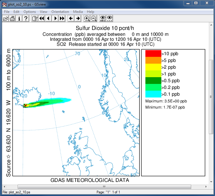
Gaseous air concentrations are normally display in volume units such as parts per million. HYSPLIT does have an option to perform the conversion to mass mixing ratio using namelist option ICHEM=6 which divides the air concentrations by the density of air (kg/m3). However, currently there is no way to set two different ICHEM options with the same simulation. Therefore, the mixing ratio correction must be estimated, which in this case we will assume is close to one because the density of air near the ground is about 1 kg/m3. Then the conversion of mass mixing ratio to volume mixing ratio is simply the ratio of the molecular weight of air (29 g/Mol) to that of the pollutant (64 g/Mol) or a ratio of 0.453. Multiplied by 1.0E+09 converts L/L to parts per billion (ppb). See the basic tutorial for a more complete discussion of mass to volume conversions. The resulting command line for the graphic display follows:concplot concentration plotting program -ivolcano.bin HYSPLIT binary output file -oplot_so2 Postscript output file -x0.453E+09 conversion kg to µg -s1 select species #1 -k2 no contour lines between colors -c4 force contour levels -v10+5+2+1+0.5+0.2+0.1 set forced contours - The simulation results show the SO2 concentrations (left) and SO4 concentrations rate for the three different conversion rates (top to bottom). This is only an example of how such a calculation can be performed. Using the particle restart option it is possible to construct a continuous emission scenario using different conversion rates with each computational segment.
SO2 SO4 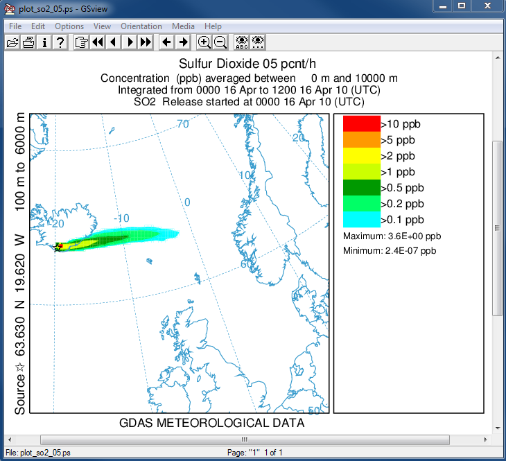

There are more complex chemical conversion modules available that work with HYSPLIT. However, these are not routinely used and the recommendation would be to work directly with the source code rather than the pre-compiled PC executables for any customized applications. For example, the sulfate conversion model was developed for acid rain applications in North America and would require some modification for application to volcanic eruptions.