2.4 Finer scale terrain and land-use (140 min)

The bdyfiles directory in the HYSPLIT installation contains three text files that provide default values for landuse, terrain, and aerodynamic roughness length in the event that they are needed and the meterological input file does not already contain those values. The three files in this directory (LANDUSE.ASC, ROUGHLEN.ASC, TERRAIN.ASC) are text files that can easily be edited. Each value is a 4-character integer on a regular latitude-longitude grid starting from the northwest corner moving east along each record and then south with each additional record. The grid corners and spacing are given in an independent file called ASCDATA.CFG. The default files provided with HYSPLIT are global at one-degree resolution. Note that these data are not always required. For instance, the landuse would only be used if the resistance deposition method or resuspension were enabled. If these data are contained in the meteorological data file, these files would not be read. The meteorological variable identification for roughness length is RGHS and SHGT or HGTS for terrain height. Currently there is no option to read the landuse variable. In this example we will replace the landuse data with a higher resolution definition of land versus water and recalculate the resuspension calculation from the last section.

1. In the previous resuspension example, deposition occurs to all surfaces, however resuspension only occurs from non-water surfaces. By increasing the resolution of the definition of land and water, we should be able to improve the calculation over Japan which is only one degree wide along the more narrow sections. The problem with the one-degree definitions is that the land boundary does not necessarily fall at even one degree intervals and we may be computing resuspension over surfaces that are clearly water. In the LANDUSE.ASC file, eleven numeric categories are defined:
   
   

   1		urban
   2		agricultural
   3		dry range
   4		deciduous
   5		coniferous
   6		mixed forest
   7		water
   8		desert
   9		wetlands
   10		mixed range
   11		rocky

   
   If you have your own data, the sample program gis2bdy is provided to reformat your land surface values to the HYSPLIT format. The input data section would need to be modified to be consistent with your data and your landuse values would need to be mapped to the ones HYSPLIT can interpret shown above. Currently there is no higher resolution HYSPLIT data available but they can easily be created from other sources. For this example calculation, the contour program was used to extract the terrain height contour from the WRF meteorological data file (wrf11031400.bin) turning on the GIS option to create a text file for a single height contour of 0.01 m to represent the island of Japan. Landuse values inside this polygon were set to 2 to represent land and values outside the polygon set to 7 to represent ocean using a resolution of 0.1 degrees (about 10 km).


2. The gis2bdy program also creates a new ASCDATA.CFG that is consistent with the data grid location and resolution. This file also defines default values for landuse and roughness length which are the values assigned to meteorological grid points that may not be in the region covered by the surface boundary files. For the example shown here, the following is required:
   
   

   33.0 135.0		lower left corner lat,lon
   0.10 0.10		grid spacing delta lat,lon
   90 80		number of grid points lat,lon
   7		default land use (water)
   0.10		default roughness length (m)
   '../files/'		location of *.ASC files



3. To ensure that the data have been correctly mapped, another program is provided called bdy2bin than will convert the surface boundary files into their HYSPLIT formatted binary equivalent, similar to a concentration file. For instance, running the program gridplot -iLANDUSE.BIN -l0 -a0 -d1 will generate the following graphics for the original 1.0-degree and 0.1-degree data:
   
   


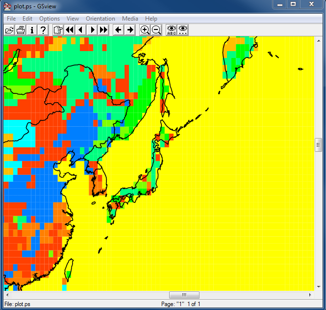
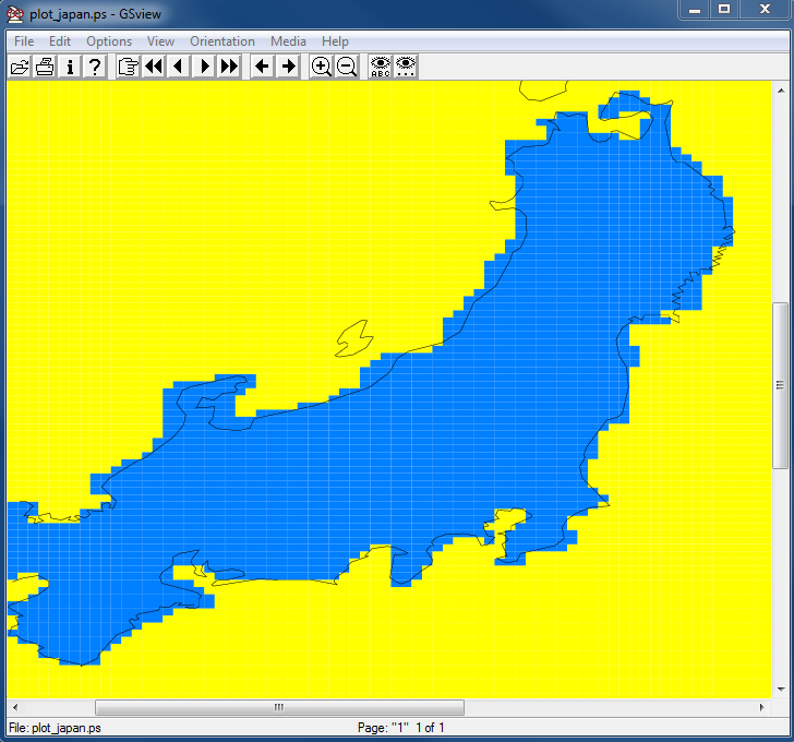
4. When the new input files have been completed, run the resuspension calculation again from the last example, using the new ASCDATA.CFG file, and you should get something similar to the following:
   
   

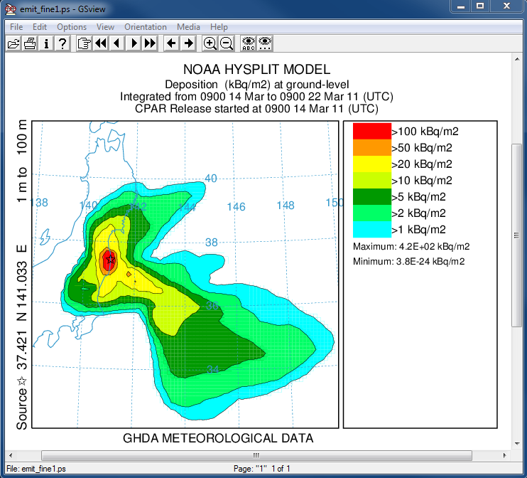
   		Total Deposition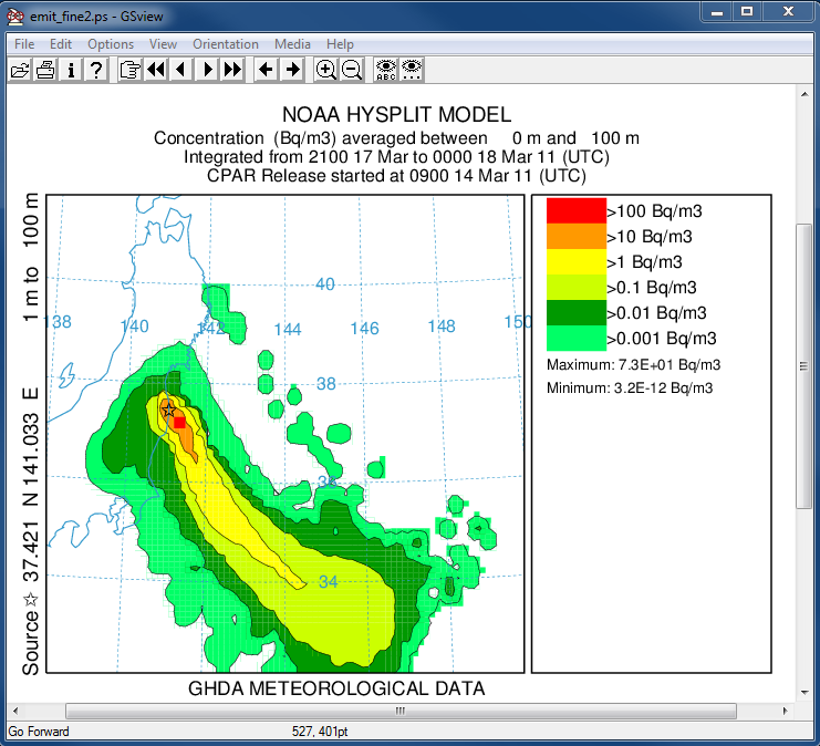
   		Air Concentration at 2100 March 17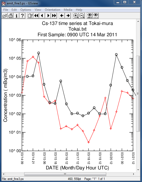
   		Time series at Tokai-mura



5. The top figure shows the total deposition pattern which is identical to the original calculation and the time series shown in the third frame is almost identical to the original time series. However, the middle frame, the air concentrations, show a much smaller emission from the high deposition grid cell to the north of Fukushima, presumably due to a greater water coverage over the higher deposition regions.

In this example, we replaced the default low-resolution global one-degree landuse file with a regional higher resolution data file and demonstrated the effect on the resuspension calculation. Not all calculations will be sensitive to changes in the surface boundary files. The HYSPLIT default is to use terrain height and roughness length from the input meteorological data if they are available.