2.3 Resuspension of deposited material (180 min) |
||||
 Previous |
|
|
 Next |
|


Under certain conditions pollutants that have deposited can be resuspended into the atmosphere if the winds are sufficiently strong and the material is not bound to the surface. Pollutant resuspension is parameterized using a pollutant resuspension factor that represents the ratio of the pollutant concentration in air C, to the amount deposited on the surface S, such that
- K = C / S,
- K = (R/S) dS/dt,
- dS/dt = k u* K S.
- Because particles will be emitted from every concentration grid cell with deposition, the computational time can become quite significant as the simulation progresses. Many of the settings are optimized to minimize the run time. The SETUP.CFG namelist file is configured for a 3D particle calculation using an release rate of 2000 particles per hour (negative = per hour) and with a maximum particle duration of 12 hours. The emission file points to the one used in previous examples for Cs-137 emissions from Fukushima:
delt = 15.0, Force time step to 15 minutes initd = 0, 3D particle calculation khmax = 12, Delete particles after 12h numpar = -2000, Release 2000 particles per hour maxpar = 1000000, maximum particle number efile = '../files/EMITIMES', Cs-137 emission rate for Fukushima - As in the other Fukushima examples, we start March 14th but this time run for 192 hours to more clearly see the effect of the resuspension calculation. We use the GDAS data rather than the higher-resolution WRF data because it covers a longer time period. The key sections of the CONTROL are as follows:
192 run duration ../../Tutorial/japan/ base tutorial Fukushima directory gdas11-22.bin half-degree GDAS extract for March 11-22 - To be able to resuspend deposited material and still enable finer temporal resolution for the air concentrations, two grids need to be defined. The first grid should be the deposition grid with an averaging time that covers the simulation period. Note that if the deposition grid were at a finer temporal resolution, the accumulated totals would be set to zero at the end of each period eliminating the potential for resuspension from those grid cells:
38.0 140.0 grid center 0.25 0.25 grid spacing 20.0 30.0 grid span ./ directory deposit.bin output file name 1 one level 0 deposition level always = 0 00 00 00 00 00 default start time 00 00 00 00 00 default stop time 00 192 00 sample collection duration - The air concentration grid could provide finer temporal and spatial resolution. Note that the grid resolution of the deposition grid is much coarser (0.25 deg) than what was used in previous calculations (0.05 deg). Using a finer grid only means that more grid points will be emitting particles which will take more time:
38.0 140.0 grid center 0.25 0.25 grid spacing 20.0 30.0 grid span ./ directory airconc.bin output file name 1 one level 100 average from ground to 100 AGL 00 00 00 00 00 default start time 00 00 00 00 00 default stop time 00 03 00 three-hour averaging time - To enable the resuspension algorithm, only the resuspension factor needs to be defined in the CONTROL file:
1.0 1.0 1.0 non-zero defines a particle 0.001 0.0 0.0 0.0 0.0 forced dry deposition at 0.1 cm/s 0.0 8.0E-05 8.0E-05 within- and below-cloud wet removal 0.0 no radioactive decay 1.0E-06 default resuspension factor - Because of the way the resuspension code interacts with the meteorological data and the deposition grid, the meteorological subgrid option is disabled when resuspension is turned on. This may increase run times substantially because all the data at the meteorological grid points must be processed. This can be compensated by creating an extract of the meteorological data file covering just the region of interest using the utility program xtrct_grid, which is available only through the command line. In this case we might want to restrict the meteorological grid by setting the upper right corner point to 70N 160E. This step is optional. Otherwise proceed with the simulation as it was configured in the last few steps.
- When the configuration is complete run the model two times, with and without the resuspension factor and you should get something similar to the following:
Standard Resuspension 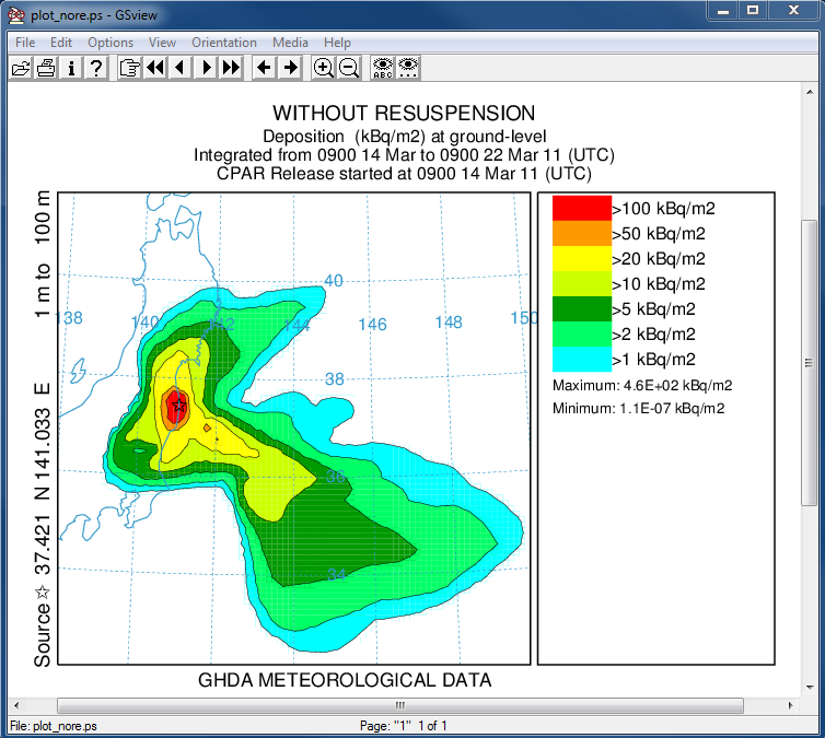
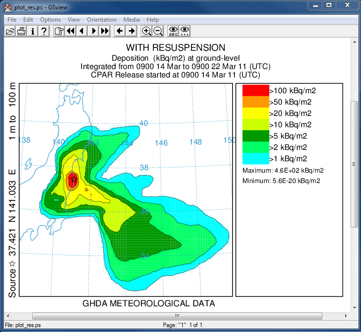
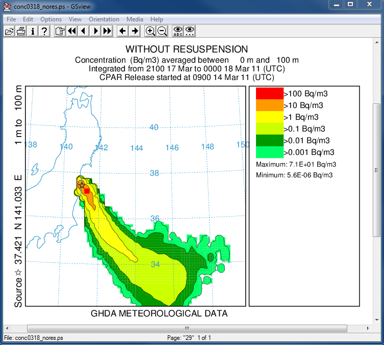
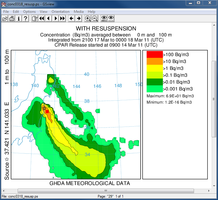
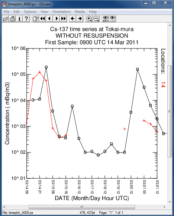
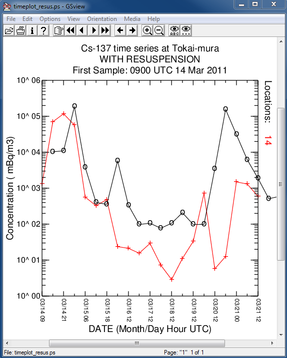
- The top figures show the total deposition pattern and with- and without resuspension appears to be identical except for the minimum concentration, which is much lower for the resuspension case because resuspended particles have much less mass and therefore subsequently deposit much less mass. The middle panels, about half-way through the simulation show the main plume from Fukushima related to the direct emissions, but one region to the north and a larger area to the south show resuspended emissions resulting in concentrations about 100-1000 times smaller than the primary release. The third panel shows the time series at Tokai-mura, about 100 km south of Fukushima, and the resuspended emissions clearly provide a baseline to the concentration predictions that is more in line with the measurements (black line) than the direct emissions only calculation.
In this example the model was configured to compute the resuspension of material deposited during the calculation. The results shown here are only intended as an example of the procedure and any application to actual conditions require a more careful selection of meteorological data and deposition parameters.