1.5 Using a TCM to compute the emissions (120 min) |
||||
 Previous |
|
|
 Next |
|


In all of the previous TCM examples the matrix attributes of the simulation were not really utilized to their full extent. Given a measurement data vector, in this case a time series of measurements at Tokai-mura, using linear algebra methods, we can find the source term vector that provides the best fit to the measurement data. Two post-processing programs are required. The first program C2ARRAY converts the unit source input files (one for each release time) into a Coefficient Matrix (CM) file so that each column represents a release time and each row a measurement location. Then the program TCSOLVE is used to find the emission rate vector.
- This application requires a one unit per hour dispersion calculation for each release period. The script for this application will recompute all the required TG_{MMDDHH} files prior to solving the matrix. The procedure for computing a multi-file TCM was reviewed in a previous section and will not be discussed in any detail below.
- The names of the individual release files need to be assembled into a list:
- dir /b TG_?????? >merg_list.txt
-
The C2ARRAY program will extract the predicted concentrations (dispersion factors) for all the emission times that contribute to each concentration measurement (location and time period) as defined in the DATEM formatted input file. The model dispersion prediction is put into its appropriate row and column of the comma delimited output file. The DATEM format is a standard format used at NOAA-ARL for a variety of different measurement data. The C2ARRAY program is called with the following command line options:
c2array program to convert TCM files into a single CM file -imerg_list.txt list of input TG files, one for each release -oc2array.csv comma delimited CM output file -m..\files\JAEA_C137.txt DATEM formatted measured data -z2 process level 2 (air concentration) of the TG input files -
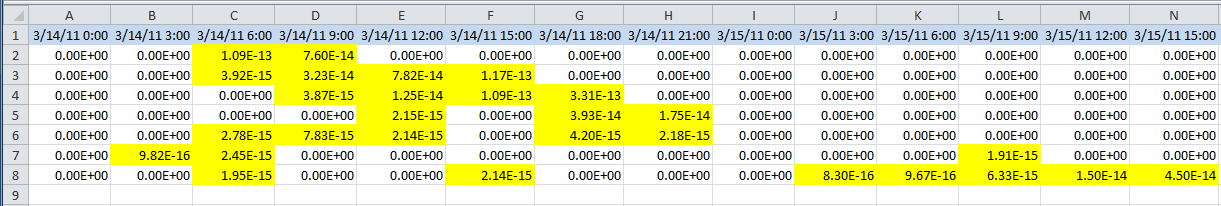
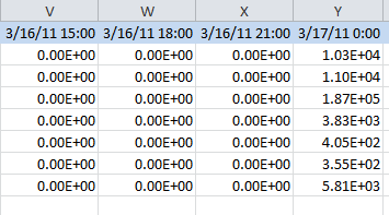
The CSV output file is shown below after import into Excel. Column headings are time in days from the year 1900. The column emission time headings (blue) were converted to a date format by Excel. The value in each row under a column shows the contribution of that release time to the measured concentration shown at the rightmost column (Y). The sum of all the columns for any row represents the contribution of all the emission times to that measurement. The yellow cells highlight those emission times that contributed a non-zero value to the measurements.
-
In its most general representation, concentrations at a downwind receptor (j) for an emission at time (i) can be represented by the relation:
Dij Si = Rj
such that the concentration at receptor R is the linear sum of all the contributing sources S times the dilution factor D between S and R. In the TCM calculation, we set S=1 and compute D for each emission time for all receptor locations (concentration grid). The C2ARRAY program extracts the D value at specific receptor locations. Given D and the measurement data R, we can solve for the emission rate S using the inverse of the coefficient matrix:
Si = (Dij)-1 Rj - The program TCSOLVE is used to solve the coefficient matrix. The units of the measurement data are arbitrary, but unit differences between the model dispersion factors (Bq) and the measurements (mBq) need to be applied to the source term vector solution, in this case a factor of 1000. Normally one would not always expect a solution due to model and measurement errors or matrix singularities, measurement data that have no contributions from any emission period. In addition, the matrix may be ill-defined, either too many equations or too few equations (measurement data). It may be necessary to manually edit the CM prior to attempting a solution. If the matrix is square, it can be solved in EXCEL using the inverse and multiplication functions.
tcsolve solves the coefficient matrix -ic2array.csv input CM array (D) -u0.001 convert R from mBq to Bq -otcsolve.txt source term solution in Bq 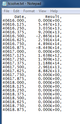
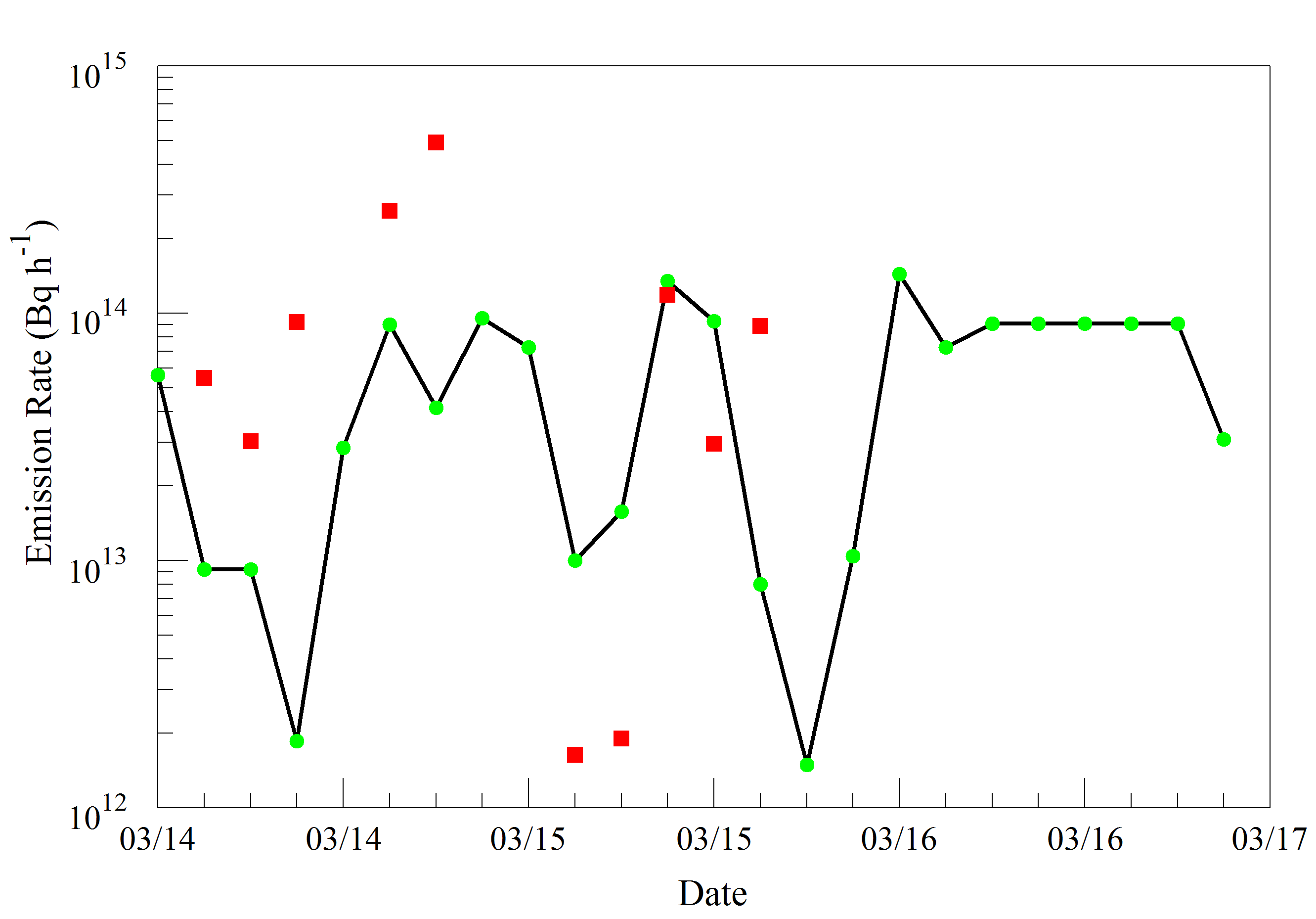
The source term vector, corresponding to each column of the CSV file is written to the output file TCSOLVE.TXT. The results are also illustrated in the graphic which shows the source term solution vector in red and the actual source term used in all the previous calculations as the green points. The negative values are not shown. Those times also roughly correspond with the plume moving away from the monitoring location resulting in greater uncertainty in the model predictions as well as whether those measurements are directly from the source or the result of previous emissions not modeled.