1.4 Updating a transfer coefficient matrix (120 min) |
||||
 Previous |
|
|
 Next |
|


In a previous example we created a Transfer Coefficient Matrix (TCM) by running a unit-source dispersion calculation for each emission period over the time period of interest. This approach is best applied to historical simulations. However, during a real-time event HYSPLIT can be configured to provide a continuous update to the TCM with each new forecast cycle by first updating the pollutant particles to the current forecast initialization time. The current-time particle positions can then be used to create a dispersion forecast if desired. For these calculations we assume the emissions and concentration output are defined every three hours. To simplify the example, only one meteorological file is used. In a real-time operational setting, the meteorological analysis data and forecast data files need to be properly associated with each simulation.
- In a previous example, the simulation for each emission was run for the entire period of interest. However in this case all simulations are divided into 3-hour segments. For example, if the first emission starts 1400 (DDHH), that simulation would end at 1403. At 1403 we start a new emission to end at 1406, but also continue the 1400 emission to end at 1406. Every three hours, we would be running an additional simulation. Particles are only released during the initial simulation, a restart simulation has no new emissions and only continues with the particles released during the release phase calculation. To perform this type of calculation, a particle position file (PARDUMP) must be written at the end of each simulation. The SETUP.CFG namelist file should contain the additional variables shown below:
ndump = 3, output particle position file after 3 hours khmax = 9999, delete particles after 9999 hours (essentially no delete) - There will be two CONTROL files, one for the particle release simulation and one for the restart simulation. They are almost identical except that in the release simulation a unit source rate for three hours is defined and the restart simulation the release rate is zero for a duration of zero. In addition, the name of the concentration output file should reflect the release time {DDHH} and sample start time {ddhh}.
New-start Simulation (particle release)
1 one pollutant CPAR defined as a Cesium Particle 1.0 emission rate of one units per hour 3.0 emission duration 3 hours each cycle CG_03{DDHH}_{DDHH} release start = sample start time
Re-start Simulation (no particle released)
1 one pollutant CPAR defined as a Cesium Particle 0.0 emission rate of one units per hour 0.0 emission duration 3 hours each cycle CG_03{DDHH}_{ddhh} release start and sample start different - The simulations are scripted to be run sequentially for each release time. In an operational setting, the script would only be run once with each new forecast cycle. In this example, only three days are simulated:
- for DD in (14 15 16) do (
- for HH (00 03 06 09 12 15 18 21) do (
At the end of each simulation, the particle output file needs to be renamed to reflect the particle release time:- rename PARDUMP PARDUMP_{DDHH}
Prior to the re-start simulation, the particle output file for that release time needs to be renamed to the default name used for input:- rename PARDUMP_{DDHH} PARINIT
- The 3-hour simulations for each release and sampling period for the above example would have created 300 CG_03{DDHH}_{ddhh} files which represent 24 release periods. In this step these files are combined into one file per release period that contains all the sampling periods. This is accomplished using another loop to go through each release time and find all the sampling files for that time and then use the program CONAPPEND to merge the files in the list to a singe file named TG_03{DDHH}:
- dir /b CG_03{DDHH}_???? >conc_list.txt
- conappend -iconc_list.txt -oTG_03{DDHH}
- The multi-file TCM structure uses the program CONDECAY to apply a time-varying release rate to the twenty four TG_03{DDHH} processed files. The program reads these files and associates the column number in the emissions file with the species index number in the HYSPLIT file and applies radioactive decay from the decay start time according to the half-life specified. Using this approach, multiple species can be processed. For a single species within the HYSPLIT input file, multiple species can be written to the output file, one output species for each group (- prefix) defined on the command line. Other arguments use the + prefix. Output file names default to DG_03{DDHH}. However, only 17 output files will be created because not all release files are associated with an emission rate. In this particular case, we use column #3 of the cfactors.txt emission file:
condecay apply emission rates to multiple files -3:1:11025.8:C137 emission column 3 = species 1 = 11025.8 days = Cs-137 +t031106 decay start time (when fission stopped) +e..\files\cfactors emission rate file +iTG_ input file prefix +oDG_ output file prefix - The final step is to merge the individual release files into a single file using the program CONMERGE. The procedure is similar to the CONAPPEND application. The final result is a single file fdnpp.bin that contains all releases and sampling periods using the defined emission profile.
- dir /b DG_?????? >merg_list.txt
- conmerge -imerg_list.txt -ofdnpp.bin
- In the first post-processing step, the model predicted concentration time series at Tokai-mura, about 100 km south of the FDNPP, is compared with the measurements:
c2datem convert model output to DATEM format -ifdnpp.bin HYSPLIT binary output file -oTokai.txt HYSPLIT DATEM output at Tokai -m..\files\JAEA_C137.txt measured data file in DATEM format -c1000.0 conversion from Bq to mBq -z2 select level #2 from input file 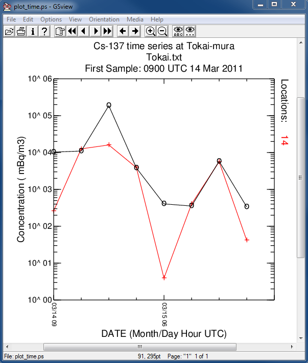
- In the second post-processing step, we create a plot of the total deposition:
concplot concentration plotting program -ifdnpp.bin HYSPLIT binary output file -oplot_dept Postscript output file -h37.0:140.0 location of map center -g0:500 radius of the map -y0.001 convert Bq to kBq -ukBq set units label on map -b0 -t0 process input data from bottom and top level 0 -k2 do not draw contour lines between colors -c4 force contour levels -v1000+500+200+100+50+20+10 set forced contours -r3 plot only the total accumulated deposition 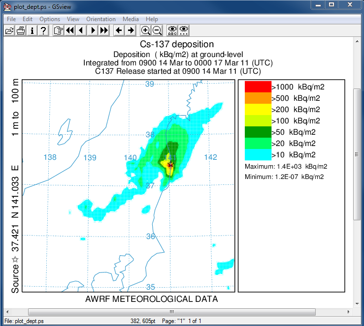
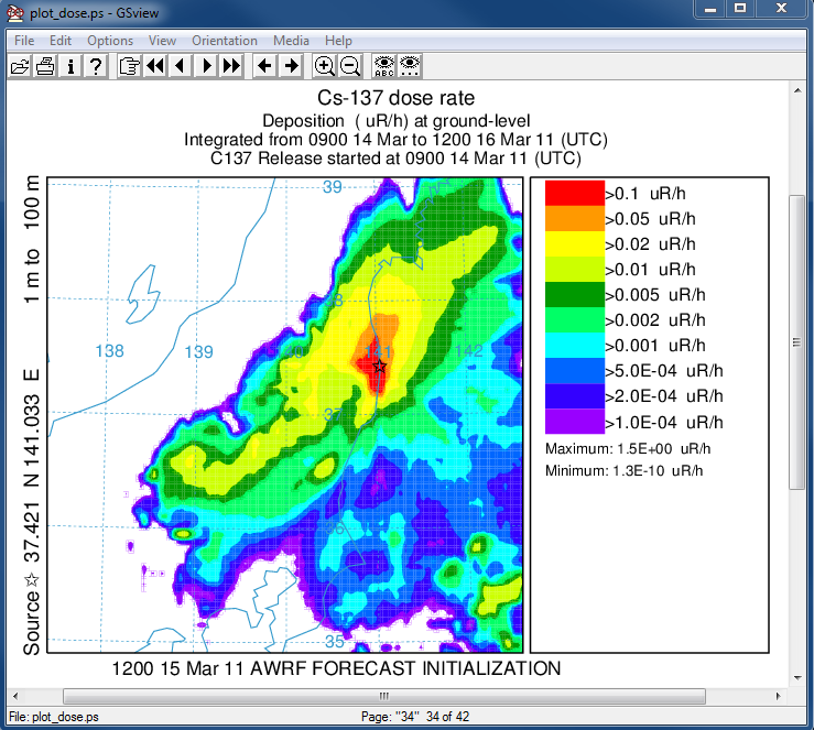
- In the last post-processing step we convert the air concentrations and accumulated deposition at each 3 hour output period to dose using the concentration plotting program. For this conversion we assume that the conversion factors are 3.3x10⁻¹¹ and 1.1E-12 (rem/h per Bq/m3 or per Bq/m2). Only the last time period is shown below:
concplot concentration plotting program -ifdnpp.bin HYSPLIT binary output file -oplot_dose Postscript output file -h37.0:140.0 location of map center -g0:500 radius of the map -x3.340E-05 convert air concentration to µrem/h -y1.08E-06 convert deposition to µrem/h -k2 do not draw contour lines between colors -c4 force contour levels -v0.1+0.05+0.02+0.01+0.005+0.002+ 0.001+0.0005+0.0002+0.0001 set forced contours -r2 sum deposition each time period 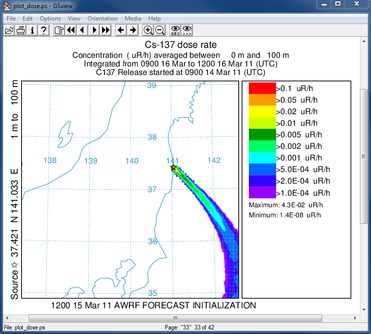
This section described how a TCM can be computed incrementally as the release progresses, updating the particle position from previous releases with each meteorological data update. Although not shown in this example, after an update has completed, another simulation can be conducted using just forecast meteorological data to project all the previous releases into the future by using the PARDUMP_{DDHH} file to initialize the forecast for each release time. The update process is trivial to parallelize because each release simulation is independent of the others and can be conducted simultaneously on multiple processors.