When multiple simulations are conducted, each one representing a different emission, the model results can be analyzed to determine which simulation provides the best fit with any available measurements, or more specifically, what emission rate is required with each simulation to provide the best fit with the measurements. These simulations can each represent a different emission time or location or a combination of both. Currently the code is configured to automatically generate multiple time-varying emissions using the namelist parameters QCYCLE and ICHEM.
As an example, if hourly (the minimum) resolution is desired over a 24 hour simulation period, then the emission rate needs to be set to emit one one unit for a duration of one hour. The namelist variable QCYCLE should also be set to 1.0 hour so that the emissions effectively become continuous at a rate of one unit per hour. This in combination with ICHEM=10 will result in the creation of 24 concentration arrays with each particle being tagged according to its release hour and those particles will only contribute to concentrations on the grid with the same release-time tag. The pollutant identification field is used and its value corresponds to hours and tenths (no decimal) after the start of the simulation. Only 4 digits are available which limits the duration to 999.9 h. The output concentration grid will appear to be like any other but with 24 pollutants, one for each release period as defined by the QCYCLE parameter. Make sure that a sufficient number of particles have been released to provide consistent results for all time periods.
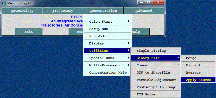
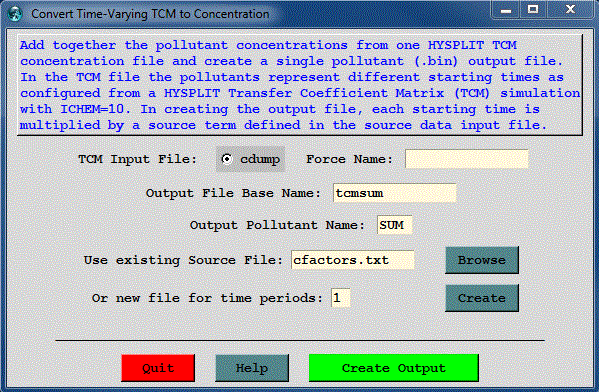
Once the simulation has completed, the unit source simulation can be converted to concentrations by applying an emission rate factor for each release time. This is accomplished by clicking on the Concentration / Utilities / Binary File / Apply Source menu tab. This menu is only intended to work with a single multi-pollutant concentration file created in the manner described previously.
The input required is simply the name of the Transfer Coefficient Matrix (TCM) input file (the previously created multi-pollutant=multi-time-period) input file, the base name of the single pollutant output file which will contain the concentration sum of all the release periods after they are multiplied by the source term, the 4-character pollutant identification field, and the name of the time-varying source term file it it exists, otherwise a new file can be created. An emission rate needs to be defined for each release time, otherwise it is assumed to be zero.
The emissions file format is simply the starting time of the emission given by year, month, day, and hour, and the emission rate in terms of units per hour. The first record of all emissions file should contain the column labels then followed by the data records, one for each release time period. For example, a constant emission rate corresponding to the 12 hour example test simulation (16 October 1996) would appear as follows:
Command Line Options - tcmsum
The underlying binary file conversion program can be run from the command line. As with all other applications, the command line argument syntax is that there should be no space between the switch and options. The command line arguments can appear in any order:
tcmsum -[option {value}]The procedure described in this section is very similar to the transfer coefficient solution approach with the exception that here the dispersion coefficients for the individual release times are contained in a single file while in the other approach an input file is required for each release time simulation. The single file created here can be processed through the utility program conlight to extract one time period to its own file with each pass through the program. Currently no GUI script application exists to perform this task automatically.