Summary: This menu is used to configure the model to execute a script to run multiple iterations of the backward trajectory calculation for periods that correspond with individual measured sampling data. The trajectory results can then be overlaid using the frequency plot menu option to indicate the most probable source regions. The CONTROL file should have been previously defined for a forward calculation that corresponds to the sampling period of the measured data. The measured data file must be in the DATEM format. The configuration process is very similar to that described for dispersion simulations.
Step 1: defines the measured data input used in this series of calculations. The trajectory model is run backward, from each of the sampling locations, for each sampling period with a non-zero measurement. Measured values less than or equal to the value in the text entry box are considered to be zero. By default, three trajectories are started for each sample, one at the beginning, middle, and end of the period. However, any starting trajectory combination can be selected using the checkboxes.
Sampling data files are in the ASCII text DATEM format. The first record provides some general information, the second record identifies all the variables that then follow on all subsequent records. There is one data record for each sample collected. All times are given in UTC.
An example measured data file can be used with the sample meteorological data to configure multiple trajectory simulations starting on 95 10 16 00. Note that the sampling data run from 0600 on the 16th through 1200 on the 17th, suggesting at least a 30 h if not 36 h trajectory is required to span the measurement data domain. First create a CONTROL file by running a forward simulation for one trajectory that spans the computational period.
Step 2: creates three CONTROL.{xxx} files for each sampling location with a non-zero measurement at the beginning, middle, and end of the sampling period using the dat2cntl program. The CONTROL files are numbered sequentially from 001 to a maximum of 999. The trajectory output files are labeled using the base name from the CONTROL file followed by the sampler ID number and the starting date and time of the trajectory. A sampler collecting two contiguous in-time samples will have the same trajectory computed at the end of one sampling period and the beginning of the next sampling period because there will be two different CONTROL files for each. However, the output file name will be the same and hence the results will not be double counted in any statistical analysis. Using the sample data, running step two creates 45 CONTROL files from 15 non-zero measurements.
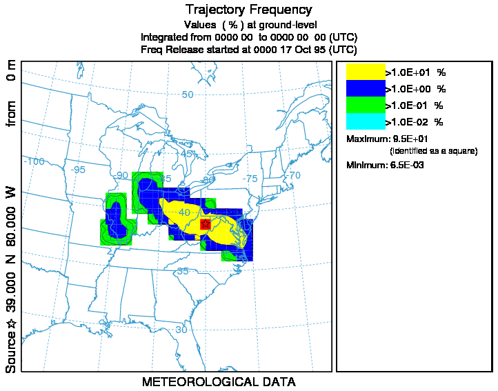
Step 3: sequentially runs the trajectory simulations starting with CONTROL.001 through the last available control file. Each simulation uses the same namelist configuration. Once the calculation has completed, the individual trajectories can be gridded and displayed using the trajectory frequency menu, the results of which are shown below.
In this case the measurement data were created using a forward dispersion simulation from 40N 80W which is near the maximum point of the trajectory frequency plot, the position of the maximum is also indicated along the left edge plot label.