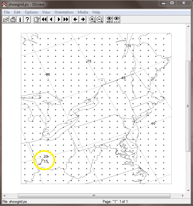
 | Meteorological data such as wind direction, speed, temperature, moisture, are provided on a regular spaced grid at multiple levels in the atmosphere. In this illustration, only every 10th grid point is displayed. The values at the grid point near Dayton, Ohio are shown in the example. |
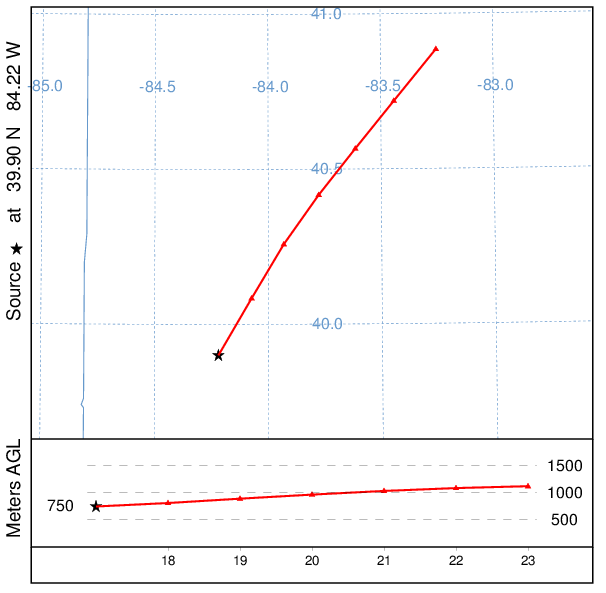 | A trajectory is the path of a single hypothetical point that is carried passively with the mean wind. The meteorological data are updated at each integration step. In this example, started at Dayton, Ohio, end-points are shown each hour for both the horizontal and vertical projections. |
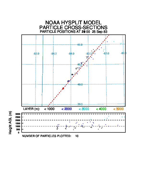 | Dispersion is introduced by calculating the trajectory for many points. However, each trajectory is perturbed by the random atmospheric turbulence along its path. In this example, 10 particles were released from Dayton, and their position is shown each hour. Note how they depart from the mean trajectory path, in both the horizontal and vertical. Higher particles travel with faster winds. |
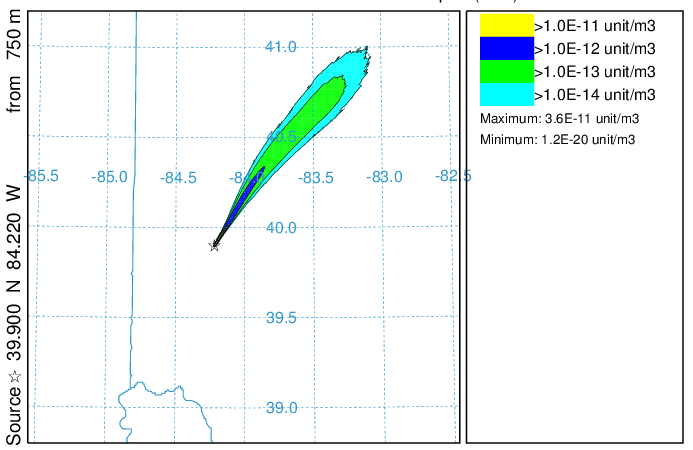 | Air concentrations are computed by adding together the mass of the computational particles and dividing by the volume of their horizontal and vertical distribution. In this example, the particle average was taken over 6 hours, the duration of the calculation, and the total particle mass was one, a unit emission. |