Time Variation of Emissions using the Ratio Method

Use the existing coefficient matrix with the 9 emission times

• Under each release time define the slope function
• Let measured data (last column) become Y
• Let model prediction (release time column) become X
• Use $Column$Row definition to fix the measured data column
• Copy slope equation to the bottom of each release column
• Show slope (M/C) solution foe each release time

Emission results for hours 15 to 23 ...

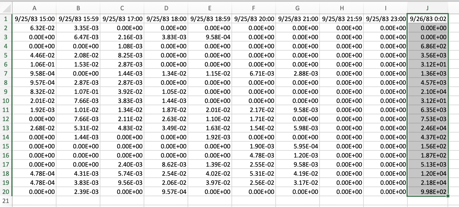
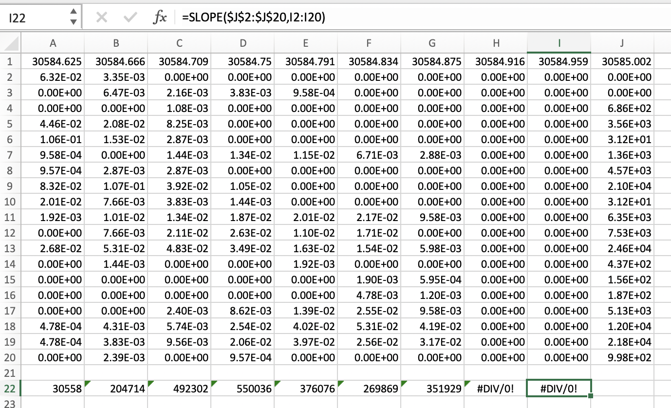
The highest emission rates are for hours 17, 18, and 19 (columns C, D, and E), and although some are almost ten times the actual emissions (67,000), they correspond with the times of the known emissions. The other approaches (SVD & Cost) seem better at resolving the non-emission periods. Although if you compute the correlation for each column, the highest values correspond to the known emission periods.

The Effect of Reducing Model Error

From Exercise #12 reduce vertical mixing
Edit src_coef.{bat|sh}

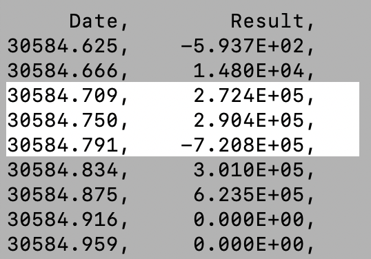
SVD kblt=1	SVD default

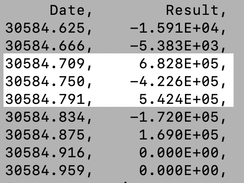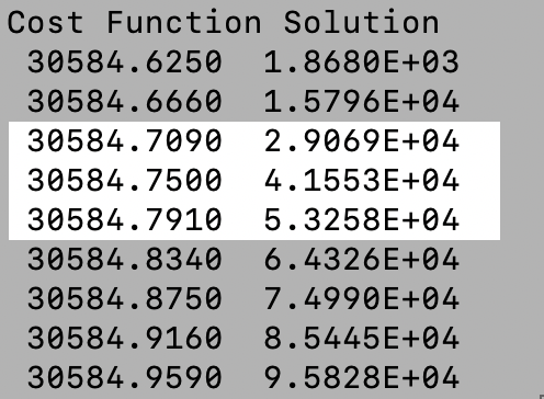
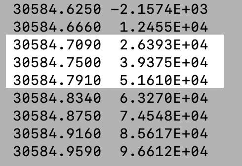
Cost function kblt=1	Cost function default

Although one would expect that the optimized simulation from the physics ensemble would reduce model errors and result in better estimates of the emissions, this was not entirely the case. The cost function solution was less sensitive to model errors as both solutions were very similar. The SVD solution seemed slightly worse showing more under-prediction, but showed better correspondence with the temporal variations than the cost function solution. Emission estimates are not only sensitive to how well the model performs at locations with above background measurements but also at those locations where only background values were observed. In many of these examples, the sensitivity to the model results is amplified by the low number of measurement data.