17.5 Configuring STILT options in HYSPLIT |
||||
 Previous |
|
|
 Next |
|
An earlier version of the HYSPLIT code was modified by Lin et al. (2003 - JGR, VOL. 108, NO. D16, 4493, doi:10.1029/2002JD003161) to optimize the application of the model to determine the CO2 fluxes over a large area based upon a backward advection-dispersion calculation from a few measurement points. This HYSPLIT modification is called the Stochastic Time-Inverted Lagrangian Transport (STILT) model and it is used to calculate a footprint field [ppm/(micro-mole/m2/s)] to represent the flux:
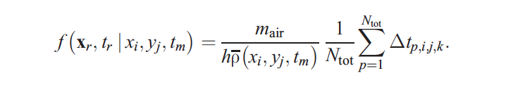
where m is the molar mass of air, ρ is the average density below h, and h is half the mixed layer depth. The summation represents the time that N particles spends in the lower half of the mixed layer. The use of STILT for inverse footprint calculations will not be addressed in this tutorial because more detailed instructions are available elsewhere.
Configuration: When HYSPLIT is configured in the STILT mode (ichem=8) the mass summation is divided by air density resulting in a mixing ratio output field and the lowest concentration summation layer (concentration layer top depth) is permitted to vary with the mixed layer depth. Although any option is permitted, if not already defined in SETUP.CFG, several other namelist parameters are automatically set as follows:
- Mass consistent dispersion,
- Hanna turbulence equations,
- Modified Richardson number,
- Variable Lagrangian time scale,
- Grell convective mixing,
| IDSP=2 | |
| KBLT=5 | |
| KMIXD=3 | |
| VSCALES=-1.0 | |
| CAPEMIN=-2.0 |
Output: When running in STILT mode, the source surface flux values at each time step (or interval OUTDT) will be output to files PARTICLE.DAT and PARTICLE_STILT.DAT. The file PARTICLE.DAT is an earlier version with the output variables fixed. While the output variables in PARTICLE_STILT.DAT are defined by the user through the namelist variables IVMAX and VARSIWANT. The surface flux output of PARTICLE.DAT represents particles that were below 50% of the mixed layer height while the output of PARTICLE_STILT.DAT represent particles that were below a user defined height (VEGHT). Some additional STILT specific namelist parameters are discussed in the model documentation provided with the code:
- TLFRAC,
- NTURB,
- VEGHT,
- ZICONTROLTF,
- WINDERRTF,
- IVMAX,
- VARSIWANT,
| fraction of the Lagrangian timescale | |
| turbulence on/off | |
| fraction of PBL for particle tally | |
| height error flag for PBL | |
| wind error flag | |
| number variables to print | |
| variable list to print |