Overview: This menu can be used to solve the transfer coefficient matrix for the source term vector given a measured data vector and where the matrix values are the dilution factors for each source-receptor pair. The measured data vector at multiple receptor locations and/or times is required and it must be defined in the DATEM format. The format of this file is discussed more detail in the GeoLocation menu. If a time-varying source solution is required, the Run Daily menu can be used to generate the required dispersion simulations. Due to model errors and insufficient sampling not all simulations will yield a solution. Results are written to the file source.txt.
Theory:Assume that the concentration at receptor R is the linear sum of all the contributing sources S times the dilution factor D between S and R:
The dilution factors are defined as the transfer coefficient matrix. The sum of each column product SiDij shows the total concentrations contributed by source i to all the receptors. The the sum of the row product SiDij for receptor j would show the total concentration contributed by all the sources to that receptor. In this situation it is assumed that S is known for all sources. The dilution factors of the coefficient matrix are normally computed explicitly from each source to all receptors, the traditional forward downwind dispersion calculation.
In the case where measurements are available at receptor R and source S is the unknown quantity, the linear relationship between sources and receptors can be expressed by the relationship:
which has a solution if we can compute the inverse of the coefficient matrix:
For example, in the case of an unrealistic 2x2 square matrix (the number of sources
equals the number of receptors), the inverse of D is given by:
| +D22 -D12 | 1/(D11D22-D12D21)
| -D21 +D11 |
The solution for S1 (first row) can be written:
As a further simplification, assume that there is no transport between S1 and R2(D12 = 0), and then the result is the trivial solution that the emission value is just the measured concentration divided by the dilution factor:
The matrix solution has three possibilities. The most common one is that there are too many sources and too few receptors which results in multiple solutions requiring singular value decomposition methods to obtain a solution. The opposite problem is that there are too many receptors and too few unknowns hence an over determined system requiring regression methods to reduce the number of equations. Unfortunately, possibilities for a matrix solution may be limited at times due to various singularities, such as columns with no contribution to any receptor or measured values that have no contribution from any source. The solution to these problems is not always entirely numerical as the underlying modeling or even the measurements can contain errors. Note that large dilution factors (very small predicted concentrations) at locations with large measured values will lead to large emissions to enable the model prediction to match those measurements. The opposite problem also exists in that negative emission values may be required to balance high predictions with small measurements. The solution to the coefficient matrix is driven by errors, either in the measurements, the dispersion model, or the meteorological data.
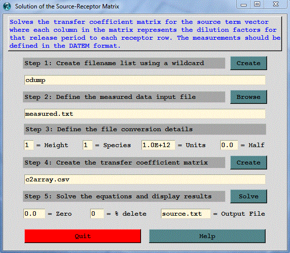
Step 1: defines the binary input files which are the output file from the dispersion simulations configured to produce output at an interval that can be matched to the measured sampling data. Ideally the model simulation emission rate should be set to a unit value. Each simulation should represent a different discrete emission period. For example, a four day event might be divided into 16 distinct 6-hour duration emission periods. Therefore the matrix would consist of 16 sources (columns) and as many rows as there are sampling data. The entry field in step 1 represents the wild card string *entry* that will be matched to the files in the working directory. The file names will be written into a file called INFILE. This file should be edited to remove any unwanted entries.
Step 2: defines the measured data input file which is an ASCII text file in the DATEM format. The first record provides some general information, the second record identifies all the variables that then follow on all subsequent records. There is one data record for each sample collected. All times are given in UTC. This file defines the receptor data vector for the matrix solution. It may be necessary to edit this file to remove sampling data that are not required or edit the simulation that produces the coefficient matrix to insure that each receptor is within the modeling domain.
Step 3: defines the file conversion details from sampling units to the emission units. For instance, the default value of 10+12 converts the emission rate units pg/hr to g/hr if the sampling data are measured in pg/m3 (pico = 10-12). The exponent is +12 rather than -12 because it is applied in the denominator. The height and species fields are the index numbers to extract from the concentration file if multiple species and levels were defined in the simulation. The half life (in days) is only required when dealing with radioactive pollutants and the measured data need to be decay corrected back to the simulation start time.
Step 4: creates the comma delimited input file called c2array.csv with the dilution factors in a column for each source and where each row represents a specific receptor location. The last column is the measured value for that receptor. The column title represents the start time of the emission in days from the year 1900. This step calls the program c2array which reads each of the measured data values and matches them to the input files to extract the dilution factors from each source to that measured value.
Step 5: solves for the source vector using the SVD (Singular Value Decomposition) methods from Numerical Recipes, The Art of Scientific Computing, Press, W.H., Flannery, B.P., Teukolsky, S.A., Vetterling, W.T., 1986, Cambridge University Press, 818 p. The solution may be controlled to some extent by defining a threshold zero dilution factor, below which the dilution factors are set to zero. An alternative approach is the define a cumulative percentage dilution factor, below which an entire sampling row may be eliminated. For instance, if the % delete field contains 10, then the rows representing the lowest 10% of the dilution factors are removed. In the event the computation fails to produce an adequate solution, it may be necessary to edit c2array.csv. The solution results are written to an output file source.txt and also displayed through the GUI. A solution may contain negative values as well as extreme positive emission results. Such values are not realistic and are a result of model errors or other uncertainties. This step calls the program tcsolve.