1.1 Time varying emissions and dose (50 min) |
||||
 Previous |
|
|
 Next |
|


In this example we define the time varying emission rate for Cs-137 during the most critical two-day period during the Fukushima accident to compute deposition and enter a simple conversion factor to estimate the dose for a single radionuclide. In the following sections below we review the key features of the script.
- Given the following emissions:
create the EMITIMES file.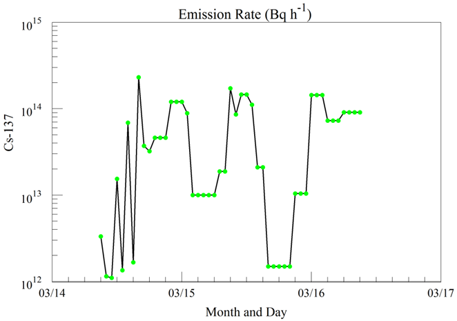
- Configure the SETUP.CFG namelist file to optimize the calculation using WRF and to speed up the computation for quicker results by deleting particles that have moved off the domain of interest:
delt = 5.0, force time step khmax = 24, delete particles after 24h numpar = -2500, release 2500 per hour maxpar = 300000, maximum particle number efile = '../files/EMITIMES', file with emission rates vscales = 5.0, stable mixing time scale vscaleu = 200.0, unstable mixing time scale kmix0 = 150, minimum mixing depth - Ensure that the emission section of the CONTROL file is set to zero to avoid using the wrong emission rate:
1 one pollutant CPAR defined as a Cesium Particle 0.0 emission rate units per hour 0.0 emission duration in hours - In the first post-processing step, the model predicted concentration time series at Tokai-mura, about 100 km south of the FDNPP, is compared with the measurements:
c2datem convert model output to DATEM format -ifdnpp.bin HYSPLIT binary output file -oTokai.txt HYSPLIT DATEM output at Tokai -m..\files\JAEA_C137.txt measured data file in DATEM format -c1000.0 conversion from Bq to mBq -z2 select level #2 from input file 
- In the second post-processing step, we create a plot of the total deposition:
concplot concentration plotting program -ifdnpp.bin HYSPLIT binary output file -oplot_dept Postscript output file -h37.0:140.0 location of map center -g0:500 radius of the map -y0.001 convert Bq to kBq -ukBq set units label on map -b0 -t0 process input data from bottom and top level 0 -k2 do not draw contour lines between colors -c4 force contour levels -v1000+500+200+100+50+20+10 set forced contours -r3 plot only the total accumulated deposition 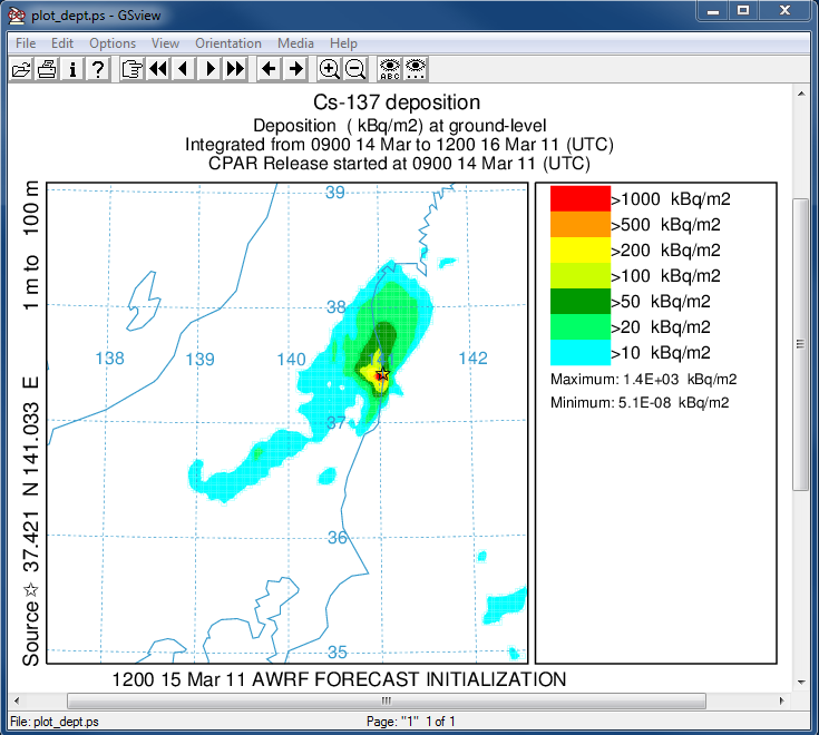
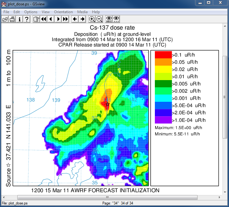
- In the last post-processing step we convert the air concentrations and accumulated deposition at each 3 hour output period to dose using the concentration plotting program. For this conversion we assume that the conversion factors are 3.3x10⁻¹¹ and 1.1E-12 (rem/h per Bq/m3 or per Bq/m2). Only the last time period is shown below:
concplot concentration plotting program -ifdnpp.bin HYSPLIT binary output file -oplot_dose Postscript output file -h37.0:140.0 location of map center -g0:500 radius of the map -x3.340E-05 convert air concentration to µrem/h -y1.08E-06 convert deposition to µrem/h -k2 do not draw contour lines between colors -c4 force contour levels -v0.1+0.05+0.02+0.01+0.005+0.002+ 0.001+0.0005+0.0002+0.0001 set forced contours -r2 sum deposition each time period 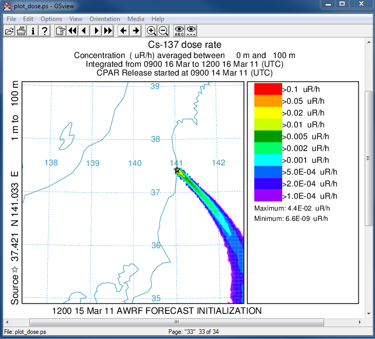
In this simple single-species HYSPLIT radiological configuration, the species characteristics, emission rate, and decay must be specified for each simulation. Although decay was not considered due to the long half life of Cesium-137, decay is only applied during the calculation for both deposition and air concentration. Once the data have been written to the output file, decay can no longer be applied. This can be mitigated by writing deposition to the output file only at the end of the simulation. However, the subsequent dose calculation will not include the fact that the average deposition during the exposure period must be some larger value than the final value written to the file. This is the primary reason why post-processing of dose calculations is recommended.