13.7 Cost Function Minimization of the CM

In the previous section the transfer coefficient matrix (TCM) and air concentration measurement data were explicitly solved for the unknown source term using matrix inversion methods. In this section, with the same TCM, we use a cost function approach to minimize the difference between the observations and model predictions by varying the source term from a first-guess estimate. The five output files from the previous section are required to continue.

1. In this example, the cost function F is minimized, q_ij are the emissions over M time periods and N source locations (in this case one location), q^b_ij is the first-guess emission estimate, σ²_ij is the emission error variance. In the second term, a^h_m and a^o_m are the HYSPLIT air concentration predictions and observations, respectively and ε²_m is the variance of the observations.
   
   

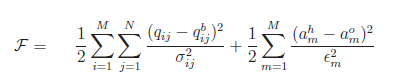
   Note that a^h_m is defined as the product of q_ij and the TCM for each release time at that observation location. Further technical details regarding the computational approach used to solve the TCM can be found in Source term estimation using air concentration measurements and a Lagrangian dispersion model–Experiments with pseudo and real cesium-137 observations from the Fukushima nuclear accident, T. Chai, R. Draxler, A. Stein, Atmospheric Environment, 106, 241-251.

2. Using the simulations from the last section for each of the five potential release times (tcm090100 - tcm090300 go to the Utilities / Transfer Coefficient tab and open the cost function menu. In step 1 replace the concentration file name wildcard with tcm and then press the Create to generate the INFILE of filenames. In step 3 define the units conversion factor and any other simulation specific requirements. Then in step 4, press Create to generate the transfer coefficient matrix in a comma delimited format.


3. Step 5 is used to create the PARAMETER_IN_000 input file for the inverse modeling executable lbfgsb. Detailed information is required that is not always well known. Several solution iterations may be required before the optimal input parameters can be properly defined. In this hypothetical example, change the first-guess source term to 1000 g/h. Leave the other parameters with their default values. If further changes are required, then consider the following:
   • The first guess value represents an estimate of the source term and the minimization will determine if there is sufficient information to change that value.
   • The scaling factor is used to reduce the numeric range of the source and predictions; a smaller range improves the solution convergence.
   • The first-guess uncertainty needs to be defined as the sum of a fraction and a constant value. The emission inversion results are less sensitive to the first guess when large uncertainties are prescribed.
   • The measurement uncertainty should also be defined as a fraction and a constant.
   • The source term solution may be bounded or unbounded. A lower bound can be used to eliminate negative solutions.
   • A logarithmic transformation can be applied to the source or the TCM results (concentrations) prior to computing a solution. The log transformation of the source also ensures non-negative solutions. In general, log transformation of the air concentrations perform better due to the large range of air concentrations.

4. In the final Step 6, run the inverse modeling executable by pressing the Solve button. The solution is displayed and the results are grams per hour. Overall the results are much better than the SVD solution with a slight under-prediction during the first two periods and the last three periods are very close to the actual emission rate of 3000 g/h.

This section demonstrates a potentially more stable alternative approach to solving the transfer coefficient matrix by varying the source term to minimize the differences between observations and model predictions because it accounts for measurement and model prediction errors. However, unlike the direct SVD solution, multiple input parameters need to be defined to achieve a solution.